def doc_theme():
    return theme_minimal() + theme(
        panel_grid_minor=element_line(color="gray", linetype="--"),
)Using Firecrown to Generate Redshift Distributions
version 1.10.0
Purpose of this document
In the previous tutorial, we explored how to use InferredGalaxyZDist objects to represent redshift distributions for galaxies. These distributions are necessary for modeling galaxy redshift distributions and can be created using various methods. In this tutorial, we will focus on generating these distributions using the ZDistLSSTSRD class in Firecrown. This class generates redshift distributions in accordance with the LSST Science Requirements Document (SRD).
The distributions for galaxies are represented by the probability density function \(P(z|B_i, \theta)\): \[ P(z|B_i, \theta) \equiv \frac{\mathrm{d}n}{\mathrm{d}z}(z;B_i, \theta), \tag{1}\] where \(B_i\) is the \(i\)-th bin of the photometric redshifts, and \(\theta\) is a set of parameters that describe the model.
In Firecrown this distribution is represented as an object of type InferredGalaxyZDist1. An object of this type contains the redshifts, the corresponding probabilities, and the data-type of the measurements. Firecrown also provides facilities to generate these distributions, given a chosen model. In firecrown.generators, we have the ZDistLSSTSRD class, which can be used to generate redshift distributions according to the LSST SRD.
1 The metadata classes described in this tutorial, unless otherwise noted, are defined in the package firecrown.metadata_types.
LSST SRD Distribution
In the LSST SRD, a redshift distribution is described by a set of parameters \(\theta = (\alpha,\,\beta,\,z_0)\), where the redshift distribution is given by \[ P(z|\theta) = f(z;\alpha,\,\beta,\,z_0) = \frac{\alpha}{z_0\Gamma[(1+\beta)/\alpha]}\left(\frac{z}{z_0}\right)^\beta\exp\left[\left(\frac{z}{z_0}\right)^\alpha\right], \tag{2}\] To obtain the distribution in each photometric redshift bin, we need to convolve this with a model for the photometric redshift errors, namely \[ P(z_\mathrm{p}|z,\sigma_z) = \frac{1}{N(z)\sqrt{2\pi}\sigma_z(1+z)}\exp\left[-\frac{1}{2}\frac{(z-z_p)^2}{\sigma_z^2(1+z)^2}\right], \tag{3}\] where \[ N(z) = \frac{1}{2}\mathrm{erfc}\left[-\frac{z}{\sqrt{2}\sigma_z(1+z)}\right]. \] The redshift distribution (Equation 1) is then given by \[ \begin{align} P(z|B_i, \theta) &= \int_{z_{p,i}^\mathrm{low}}^{z_{p,i}^\mathrm{up}} \!\!\!\mathrm{d}z_p\,P(z_p|z,\sigma_z)P(z|\theta), \\ &= \int_{z_{p,i}^\mathrm{low}}^{z_{p,i}^\mathrm{up}} \!\!\!\mathrm{d}z_p\,\frac{1}{\sqrt{2\pi}\sigma_z(1+z)}\exp\left[-\frac{1}{2}\frac{(z-z_p)^2}{\sigma_z^2(1+z)^2}\right]f(z;\alpha,\,\beta,\,z_0). \end{align} \tag{4}\] where \(B_i = \left(z_{p,i}^\mathrm{low}, z_{p,i}^\mathrm{up}, \sigma_z\right)\) provides the photometric redshift bin limits and the photometric redshift error in the form \(\sigma_z(1+z)\).
Objects of type ZDistLSSTSRD can be used to generate redshift distributions according to the LSST SRD. The following code block demonstrates how to use them to generate the redshift distributions for a given set of parameters \(\theta\).2
2 Note that the SRD fixes \(\beta = 2\). The values of \(\alpha\) and \(z_0\) are different for Year 1 and Year 10. ZDistLLSTSRD provides these values as defaults and allows for greater flexibility when desired.
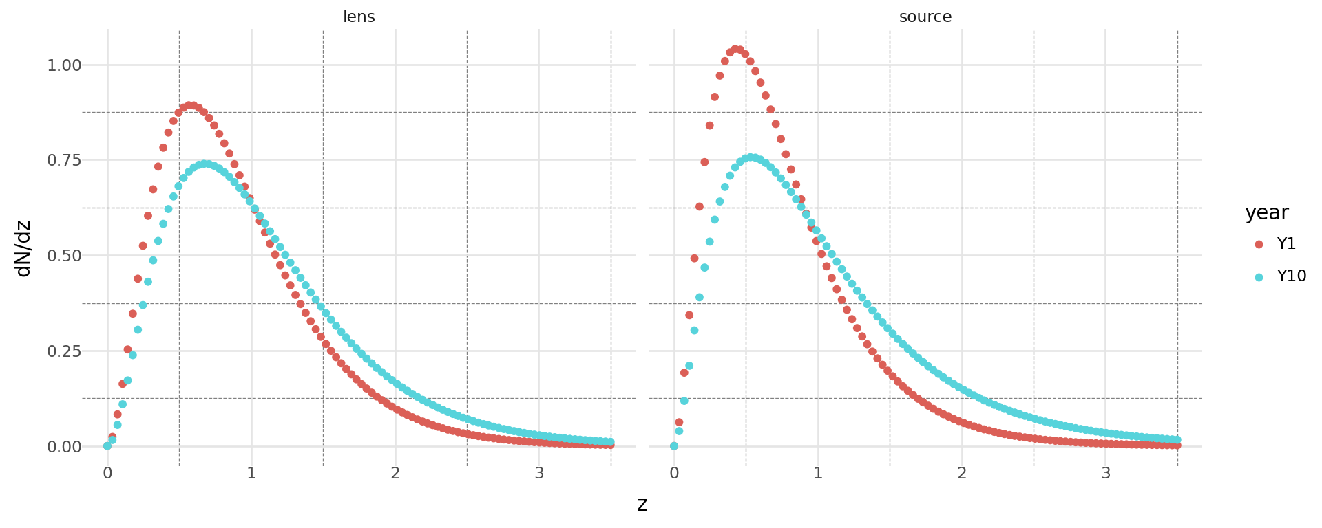
Below we calculate Equation 2 for year 1 and year 10 parameters from LSST SRD. Here we are choosing \(100\) equally-spaced points in the range \(0 < z < 3.5\) at which to evaluate the function \(f(z)\).
import numpy as np
import firecrown
from firecrown.generators.inferred_galaxy_zdist import ZDistLSSTSRD

# These are the values of z at which we will evalute f(z)
z = np.linspace(0, 3.5, 100)

# We want to evaluate f(z) for both Y1 and Y10, using the SRD prescriptions.
zdist_y1_lens = ZDistLSSTSRD.year_1_lens(use_autoknot=True, autoknots_reltol=1.0e-5)
zdist_y10_lens = ZDistLSSTSRD.year_10_lens(use_autoknot=True, autoknots_reltol=1.0e-5)

zdist_y1_source = ZDistLSSTSRD.year_1_source(use_autoknot=True, autoknots_reltol=1.0e-5)
zdist_y10_source = ZDistLSSTSRD.year_10_source(
    use_autoknot=True, autoknots_reltol=1.0e-5
)

# Now we can generate the values we want to plot.
# Note that Pz_y1_* and Pz_y10_* are both numpy arrays:
Pz_y1_lens = zdist_y1_lens.distribution(z)
Pz_y10_lens = zdist_y10_lens.distribution(z)

Pz_y1_source = zdist_y1_source.distribution(z)
Pz_y10_source = zdist_y10_source.distribution(z)
We use NumCosmo’s autoknots to determine the number of knots to use in the spline interpolation. This allows us to create the knots such that the interpolation error is less than \(10^{-5}\).3
3 The autoknots method is a part of the NumCosmo package, which is a dependency of Firecrown. See the NumCosmo documentation for more information.
The generated data are plotted in Figure 1
Code
from plotnine import *  # bad form in programs, but seems OK for plotnine
import pandas as pd

# The data were not originally generated in a dataframe convenient for
# plotting, so our first task it to put them into such a form.
d_y_all = pd.concat(
    [
        pd.DataFrame(
            {
                "z": z,
                "dndz": Pz,
                "year": year,
                "distribution": dist,
            }
        )
        for Pz, year, dist in [
            (Pz_y1_lens, "Y1", "lens"),
            (Pz_y10_lens, "Y10", "lens"),
            (Pz_y1_source, "Y1", "source"),
            (Pz_y10_source, "Y10", "source"),
        ]
    ]
)

# Now we can generate the plot. We need a theme to increase the width
(
    ggplot(d_y_all, aes("z", "dndz", color="year"))
    + geom_point()
    + labs(y="dN/dz")
    + doc_theme()
    + facet_wrap("~ distribution", ncol=2)
    + theme(figure_size=(10, 4))
)
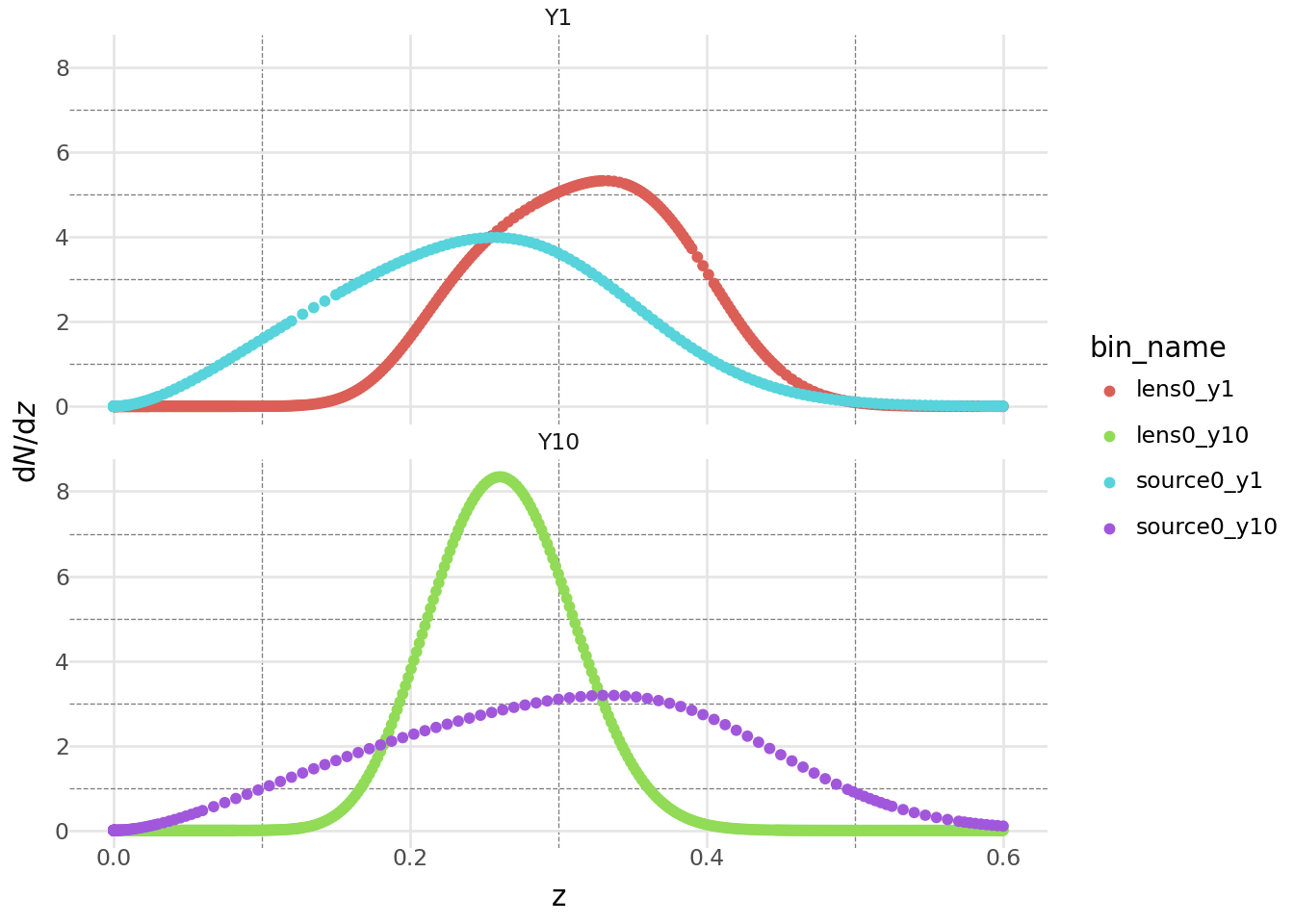
Next, using the same SRD prescriptions, we want to generate the InferredGalaxyZDist objects representing Equation 1 for a specific binning, and using a specific resolution parameter \(\sigma_z\). Here we show the first bin for the lens and source samples for both Year 1 and Year 10, the functions are evaluated at \(100\) points equally spaced between \(0\) and \(0.6\).4
4 Note that we are making use of several module-level constants in the firecrown.generators.inferred_galaxy_zdist module, namely Y1_LENS_BINS, Y10_LENS_BINS, Y1_SOURCE_BINS, and Y10_SOURCE_BINS, which are dictionaries that contain the bin edges and the resolution parameter \(\sigma_z\) for the bins.
import numpy as np
import firecrown
from firecrown.generators.inferred_galaxy_zdist import (
    ZDistLSSTSRD,
    InferredGalaxyZDist,
    Y1_LENS_BINS,
    Y10_LENS_BINS,
    Y1_SOURCE_BINS,
    Y10_SOURCE_BINS,
)
from firecrown.metadata_types import Measurement, Galaxies

# These are the values at which we will evaluate the distribution.
z = np.linspace(0.0, 0.6, 100)


# We use the same zdist_y1_* and zdist_y10_* that were created above.
# We create two InferredGalaxyZDist objects, one for Y1 and one for Y10.
Pz_lens0_y1 = zdist_y1_lens.binned_distribution(
    zpl=Y1_LENS_BINS["edges"][0],
    zpu=Y1_LENS_BINS["edges"][1],
    sigma_z=Y1_LENS_BINS["sigma_z"],
    z=z,
    name="lens0_y1",
    measurements={Galaxies.COUNTS},
)
Pz_source0_y1 = zdist_y1_source.binned_distribution(
    zpl=Y1_SOURCE_BINS["edges"][0],
    zpu=Y1_SOURCE_BINS["edges"][1],
    sigma_z=Y1_SOURCE_BINS["sigma_z"],
    z=z,
    name="source0_y1",
    measurements={Galaxies.SHEAR_E},
)
Pz_lens0_y10 = zdist_y10_lens.binned_distribution(
    zpl=Y10_LENS_BINS["edges"][0],
    zpu=Y10_LENS_BINS["edges"][1],
    sigma_z=Y10_LENS_BINS["sigma_z"],
    z=z,
    name="lens0_y10",
    measurements={Galaxies.COUNTS},
)
Pz_source0_y10 = zdist_y10_source.binned_distribution(
    zpl=Y10_SOURCE_BINS["edges"][0],
    zpu=Y10_SOURCE_BINS["edges"][1],
    sigma_z=Y10_SOURCE_BINS["sigma_z"],
    z=z,
    name="source0_y10",
    measurements={Galaxies.SHEAR_E},
)

# Next we check that the objects we created are of the expected type.
assert isinstance(Pz_lens0_y1, InferredGalaxyZDist)
assert isinstance(Pz_lens0_y10, InferredGalaxyZDist)
assert isinstance(Pz_source0_y1, InferredGalaxyZDist)
assert isinstance(Pz_source0_y10, InferredGalaxyZDist)
The plot of the \(\textrm{d}N/\textrm{d}z\) distributions in these InferredGalaxyZDist objects is shown in Figure 2.
Code
# We have already imported plotnine, so we don't need to do that again.
# This time we generate the dataframe using a different technique.
d_lens0_y1 = pd.DataFrame(
    {
        "z": Pz_lens0_y1.z,
        "dndz": Pz_lens0_y1.dndz,
        "year": "Y1",
        "bin_name": Pz_lens0_y1.bin_name,
    }
)
d_source0_y1 = pd.DataFrame(
    {
        "z": Pz_source0_y1.z,
        "dndz": Pz_source0_y1.dndz,
        "year": "Y1",
        "bin_name": Pz_source0_y1.bin_name,
    }
)
d_lens0_y10 = pd.DataFrame(
    {
        "z": Pz_lens0_y10.z,
        "dndz": Pz_lens0_y10.dndz,
        "year": "Y10",
        "bin_name": Pz_lens0_y10.bin_name,
    }
)
d_source0_y10 = pd.DataFrame(
    {
        "z": Pz_source0_y10.z,
        "dndz": Pz_source0_y10.dndz,
        "year": "Y10",
        "bin_name": Pz_source0_y10.bin_name,
    }
)
data = pd.concat([d_lens0_y1, d_source0_y1, d_lens0_y10, d_source0_y10])

(
    ggplot(data, aes("z", "dndz", color="bin_name"))
    + geom_point()
    + labs(y=r"$\mathrm{d}N/\mathrm{d}z$")
    + doc_theme()
    + facet_wrap("~ year", nrow=2)
)
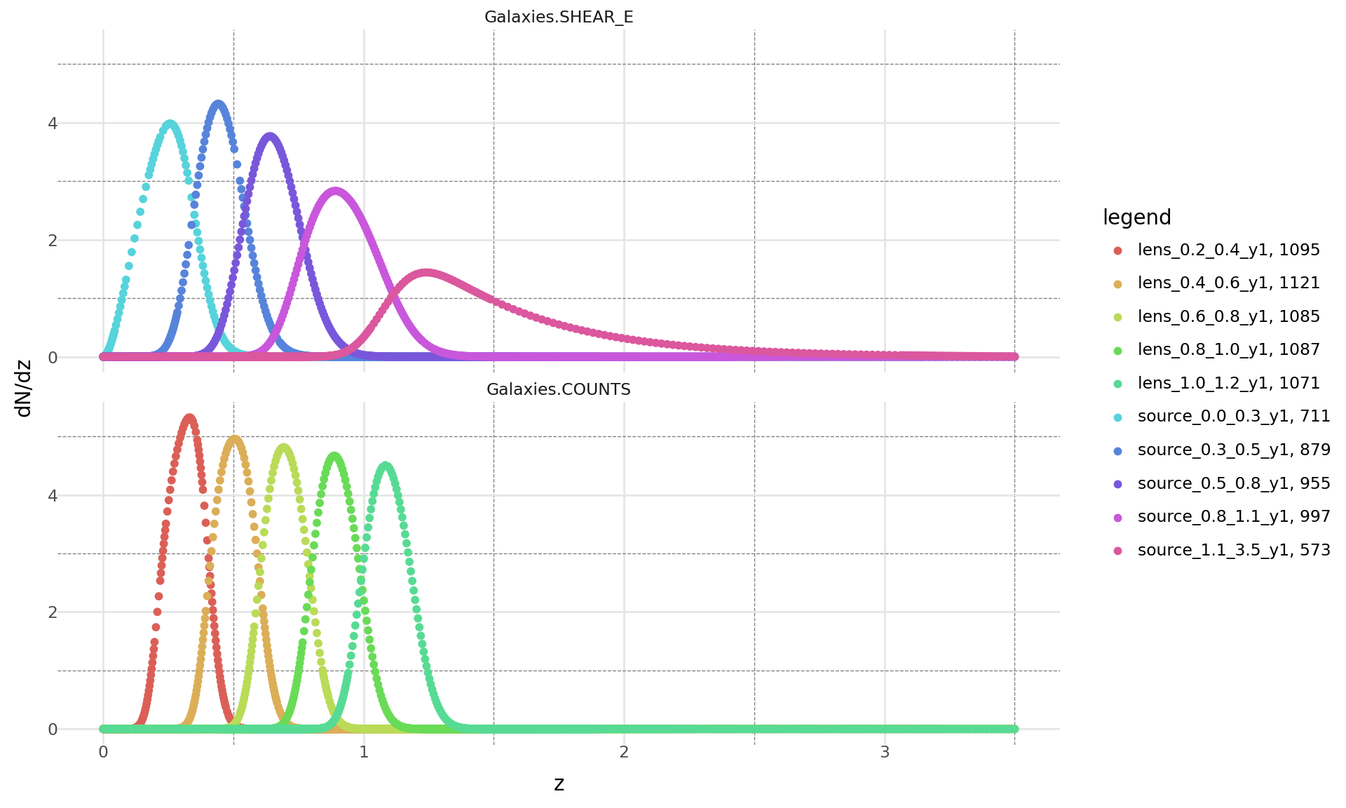
Generating the redshift distribution for all bins at once
The ZDistLSSTSRD object can also be used to generate the redshift distribution for all bins at once. The following code block demonstrates how to do this.
from itertools import pairwise

# We use the same zdist_y1 and zdist_y10 that were created above.
# We create two InferredGalaxyZDist objects, one for Y1 and one for Y10.
z = np.linspace(0.0, 3.5, 1000)
all_y1_bins = [
    zdist_y1_lens.binned_distribution(
        zpl=zpl,
        zpu=zpu,
        sigma_z=Y1_LENS_BINS["sigma_z"],
        z=z,
        name=f"lens_{zpl:.1f}_{zpu:.1f}_y1",
        measurements={Galaxies.COUNTS},
    )
    for zpl, zpu in pairwise(Y1_LENS_BINS["edges"])
] + [
    zdist_y1_source.binned_distribution(
        zpl=zpl,
        zpu=zpu,
        sigma_z=Y1_SOURCE_BINS["sigma_z"],
        z=z,
        name=f"source_{zpl:.1f}_{zpu:.1f}_y1",
        measurements={Galaxies.SHEAR_E},
    )
    for zpl, zpu in pairwise(Y1_SOURCE_BINS["edges"])
]
The plot of the \(\textrm{d}N/\textrm{d}z\) distributions in these InferredGalaxyZDist objects is shown in Figure 3.
Code
# We have already imported plotnine, so we don't need to do that again.
# This time we generate the dataframe using a different technique.
d_y1 = pd.concat(
    [
        pd.DataFrame(
            {
                "z": Pz.z,
                "dndz": Pz.dndz,
                "bin": Pz.bin_name,
                "measurement": list(Pz.measurements)[0],
                "legend": f"{Pz.bin_name}, {len(Pz.z)}",
            }
        )
        for Pz in all_y1_bins
    ]
)

(
    ggplot(d_y1, aes("z", "dndz", color="legend"))
    + geom_point()
    + labs(y="dN/dz")
    + facet_wrap("~ measurement", nrow=2)
    + doc_theme()
    + theme(figure_size=(10, 6))
)
Source Binning
The SRD specifies different binning strategies for lens and source samples. - Lens binning: Defined by explicitly providing the bin edges.
- Source binning: Defined to ensure equal numbers of galaxies in each bin.
The ZDistLSSTSRD class offers the equal_area_bins method to generate source bins with equal galaxy counts. However, the implementation involves some subtleties due to the complexity of photometric redshift distributions.
Since the final photometric redshift distribution is a convolution of the true redshift distribution with photometric redshift errors, generating bins directly from photometric redshifts is non-trivial. The process involves: 1. Generating the true redshift distribution.
2. Convolving it with photometric redshift errors to produce the final photometric redshift distribution.
3. Using the cumulative distribution function (CDF) of the photometric distribution to determine the bin edges that yield equal galaxy counts per bin.
Because this exact approach can be computationally expensive, the equal_area_bins method offers an approximate mode by setting use_true_distribution=True. In this mode, the bins are generated using the true redshift distribution only, which is faster but may not perfectly balance the galaxy counts across bins.
The following code block demonstrates how to generate source bins with equal galaxy counts using the ZDistLSSTSRD class.
# We use the same zdist_y1_source that was created above.
# Next, we generate the source bins using the true distribution.
source_bins = zdist_y1_source.equal_area_bins(
    n_bins=5, sigma_z=Y1_SOURCE_BINS["sigma_z"], use_true_distribution=True, last_z=3.5
)

# Now we do the same, but using the photometric distribution.
source_bins_phot = zdist_y1_source.equal_area_bins(
    n_bins=5, sigma_z=Y1_SOURCE_BINS["sigma_z"], use_true_distribution=False, last_z=3.5
)
We can plot just the bins edges to see the difference between the two methods.
Code
z = np.linspace(0.0, 3.5, 1000)
stats = zdist_y1_source.compute_distribution(Y1_SOURCE_BINS["sigma_z"])
dndz = np.array([stats.eval_p(z_i) for z_i in z])

d_source_bins = pd.DataFrame({"z": z, "dndz": dndz})

# Create DataFrames for the bin edges
d_bin_edges = pd.DataFrame({"bin_edges": source_bins})
d_bin_edges_phot = pd.DataFrame({"bin_edges_phot": source_bins_phot})

(
    ggplot(d_source_bins, aes("z", "dndz"))
    + geom_line()
    + geom_vline(
        data=d_bin_edges,
        mapping=aes(xintercept="bin_edges"),
        color="red",
        linetype="dashed",
        size=0.8,
    )
    + geom_vline(
        data=d_bin_edges_phot,
        mapping=aes(xintercept="bin_edges_phot"),
        color="blue",
        linetype="dotted",
        size=0.8,
    )
    + labs(y="dN/dz")
    + doc_theme()
    + theme(figure_size=(10, 4))
)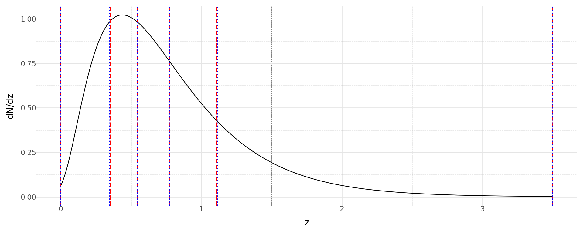
The plot in Figure 4 shows the bin edges for the source sample in LSST Year 1. The red dashed lines represent the bin edges generated using the true distribution, while the blue dotted lines represent the bin edges generated using the photometric distribution. The percentage difference in the number of galaxies in each bin is shown in the table below.
Code
N_total = stats.eval_pdf(3.5)
N_gal = np.array(
    [
        (stats.eval_pdf(zu) - stats.eval_pdf(zl)) / N_total
        for zl, zu in pairwise(source_bins)
    ]
)
N_gal_phot = np.array(
    [
        (stats.eval_pdf(zu) - stats.eval_pdf(zl)) / N_total
        for zl, zu in pairwise(source_bins_phot)
    ]
)
percent_diff = 100.0 * (N_gal - N_gal_phot) / N_gal
(
    pd.DataFrame(
        {
            "True Distribution Bin": [
                f"({i:.3f}, {j:.3f})" for i, j in pairwise(source_bins)
            ],
            "Photometric Distribution Bin": [
                f"({i:.3f}, {j:.3f})" for i, j in pairwise(source_bins_phot)
            ],
            "Galaxies (True Dist.)": [f"{n:.3f}" for n in N_gal],
            "Galaxies (Photometric Dist.)": [f"{n:.3f}" for n in N_gal_phot],
            "Percent Difference (%)": [f"{p:.1f}%" for p in percent_diff],
        }
    )
)| True Distribution Bin | Photometric Distribution Bin | Galaxies (True Dist.) | Galaxies (Photometric Dist.) | Percent Difference (%) | |
|---|---|---|---|---|---|
| 0 | (0.000, 0.352) | (0.000, 0.347) | 0.205 | 0.200 | 2.6% |
| 1 | (0.352, 0.547) | (0.347, 0.545) | 0.196 | 0.200 | -1.8% |
| 2 | (0.547, 0.771) | (0.545, 0.772) | 0.197 | 0.200 | -1.4% |
| 3 | (0.771, 1.109) | (0.772, 1.114) | 0.199 | 0.200 | -0.7% |
| 4 | (1.109, 3.500) | (1.114, 3.500) | 0.202 | 0.200 | 1.1% |
End note
Note that these facilities for creating redshift distributions are not limitations on the use of the distributions. Any facility that can create the \(z\) and \(\textrm{d}N/\textrm{d}z\) arrays can be used to create an InferredGalaxyZDist object. Code that uses the InferrredGalaxyZDist objects does not depend on how they were created.