def doc_theme():
    return theme_minimal() + theme(
        panel_grid_minor=element_line(color="gray", linetype="--"),
)Using Firecrown to Generate Two-Point Statistics for LSST
version 1.11.0a0
Purpose of this Document
In the tutorial redshift distributions we illustrate the process of using Firecrown to create redshift distributions based on specified parameters describing the distributions. Additionally, in serializable redshift distributions we demonstrate how to generate redshift distributions using serializable objects. This document outlines how to use InferredGalaxyZDist objects to derive the two-point statistics pertinent to the Large Synoptic Survey Telescope (LSST), employing the redshift distribution outlined in the LSST Science Requirements Document (SRD).
Two-point statistics
Two-point statistics are widely used in cosmological analyses. They provide a statistical summary of the distribution, in either real of harmonic space, of galaxies and the matter density field, or of other observables. In Firecrown, two-point statistics are represented by the TwoPoint class, in the module firecrown.likelihood.two_point.
Generating the LSST Year 1 Redshift Distribution Bins
Our initial step involves generating all photometric redshift bins necessary for the LSST year 1 redshift distribution. This process is detailed here in the tutorial on redshift distributions. In the serialization tutorial, we demonstrate how to get the LSST SRD redshift distributions. Here we will use the LSST SRD year 1 redshift distribution to generate the two-point statistics.
from firecrown.generators.inferred_galaxy_zdist import (
    LSST_Y1_LENS_HARMONIC_BIN_COLLECTION,
    LSST_Y1_SOURCE_HARMONIC_BIN_COLLECTION,
)

count_bins = LSST_Y1_LENS_HARMONIC_BIN_COLLECTION.generate()
shear_bins = LSST_Y1_SOURCE_HARMONIC_BIN_COLLECTION.generate()
all_y1_bins = count_bins + shear_bins
Generating the Two-Point Metadata
Within firecrown.metadata_functions, a suite of functions is available to calculate all possible two-point statistic metadata corresponding to a designated set of bins. For instance, demonstrated below is the computation of all feasible metadata tailored to the LSST year 1 redshift distribution:
import numpy as np
from firecrown.metadata_functions import make_all_photoz_bin_combinations, TwoPointHarmonic

all_two_point_xy = make_all_photoz_bin_combinations(all_y1_bins)
ells = np.unique(np.geomspace(2, 2000, 128).astype(int))
all_two_point_cells = [TwoPointHarmonic(XY=xy, ells=ells) for xy in all_two_point_xy]
The code above generates the following table of two-point statistic metadata:
Code
import pandas as pd
from IPython.display import Markdown

two_point_names = [
    (Cells.XY.x.bin_name, Cells.XY.y.bin_name, Cells.get_sacc_name())
    for Cells in all_two_point_cells
]
df = pd.DataFrame(two_point_names, columns=["bin-x", "bin-y", "SACC data-type"])
Markdown(df.to_markdown())| bin-x | bin-y | SACC data-type | |
|---|---|---|---|
| 0 | lens_0.2_0.4_y1 | lens_0.2_0.4_y1 | galaxy_density_cl |
| 1 | lens_0.2_0.4_y1 | lens_0.4_0.6_y1 | galaxy_density_cl |
| 2 | lens_0.2_0.4_y1 | lens_0.6_0.8_y1 | galaxy_density_cl |
| 3 | lens_0.2_0.4_y1 | lens_0.8_1.0_y1 | galaxy_density_cl |
| 4 | lens_0.2_0.4_y1 | lens_1.0_1.2_y1 | galaxy_density_cl |
| 5 | lens_0.2_0.4_y1 | source_0.0_0.3_y1 | galaxy_shearDensity_cl_e |
| 6 | lens_0.2_0.4_y1 | source_0.3_0.5_y1 | galaxy_shearDensity_cl_e |
| 7 | lens_0.2_0.4_y1 | source_0.5_0.8_y1 | galaxy_shearDensity_cl_e |
| 8 | lens_0.2_0.4_y1 | source_0.8_1.1_y1 | galaxy_shearDensity_cl_e |
| 9 | lens_0.2_0.4_y1 | source_1.1_3.5_y1 | galaxy_shearDensity_cl_e |
| 10 | lens_0.4_0.6_y1 | lens_0.4_0.6_y1 | galaxy_density_cl |
| 11 | lens_0.4_0.6_y1 | lens_0.6_0.8_y1 | galaxy_density_cl |
| 12 | lens_0.4_0.6_y1 | lens_0.8_1.0_y1 | galaxy_density_cl |
| 13 | lens_0.4_0.6_y1 | lens_1.0_1.2_y1 | galaxy_density_cl |
| 14 | lens_0.4_0.6_y1 | source_0.0_0.3_y1 | galaxy_shearDensity_cl_e |
| 15 | lens_0.4_0.6_y1 | source_0.3_0.5_y1 | galaxy_shearDensity_cl_e |
| 16 | lens_0.4_0.6_y1 | source_0.5_0.8_y1 | galaxy_shearDensity_cl_e |
| 17 | lens_0.4_0.6_y1 | source_0.8_1.1_y1 | galaxy_shearDensity_cl_e |
| 18 | lens_0.4_0.6_y1 | source_1.1_3.5_y1 | galaxy_shearDensity_cl_e |
| 19 | lens_0.6_0.8_y1 | lens_0.6_0.8_y1 | galaxy_density_cl |
| 20 | lens_0.6_0.8_y1 | lens_0.8_1.0_y1 | galaxy_density_cl |
| 21 | lens_0.6_0.8_y1 | lens_1.0_1.2_y1 | galaxy_density_cl |
| 22 | lens_0.6_0.8_y1 | source_0.0_0.3_y1 | galaxy_shearDensity_cl_e |
| 23 | lens_0.6_0.8_y1 | source_0.3_0.5_y1 | galaxy_shearDensity_cl_e |
| 24 | lens_0.6_0.8_y1 | source_0.5_0.8_y1 | galaxy_shearDensity_cl_e |
| 25 | lens_0.6_0.8_y1 | source_0.8_1.1_y1 | galaxy_shearDensity_cl_e |
| 26 | lens_0.6_0.8_y1 | source_1.1_3.5_y1 | galaxy_shearDensity_cl_e |
| 27 | lens_0.8_1.0_y1 | lens_0.8_1.0_y1 | galaxy_density_cl |
| 28 | lens_0.8_1.0_y1 | lens_1.0_1.2_y1 | galaxy_density_cl |
| 29 | lens_0.8_1.0_y1 | source_0.0_0.3_y1 | galaxy_shearDensity_cl_e |
| 30 | lens_0.8_1.0_y1 | source_0.3_0.5_y1 | galaxy_shearDensity_cl_e |
| 31 | lens_0.8_1.0_y1 | source_0.5_0.8_y1 | galaxy_shearDensity_cl_e |
| 32 | lens_0.8_1.0_y1 | source_0.8_1.1_y1 | galaxy_shearDensity_cl_e |
| 33 | lens_0.8_1.0_y1 | source_1.1_3.5_y1 | galaxy_shearDensity_cl_e |
| 34 | lens_1.0_1.2_y1 | lens_1.0_1.2_y1 | galaxy_density_cl |
| 35 | lens_1.0_1.2_y1 | source_0.0_0.3_y1 | galaxy_shearDensity_cl_e |
| 36 | lens_1.0_1.2_y1 | source_0.3_0.5_y1 | galaxy_shearDensity_cl_e |
| 37 | lens_1.0_1.2_y1 | source_0.5_0.8_y1 | galaxy_shearDensity_cl_e |
| 38 | lens_1.0_1.2_y1 | source_0.8_1.1_y1 | galaxy_shearDensity_cl_e |
| 39 | lens_1.0_1.2_y1 | source_1.1_3.5_y1 | galaxy_shearDensity_cl_e |
| 40 | source_0.0_0.3_y1 | source_0.0_0.3_y1 | galaxy_shear_cl_ee |
| 41 | source_0.0_0.3_y1 | source_0.3_0.5_y1 | galaxy_shear_cl_ee |
| 42 | source_0.0_0.3_y1 | source_0.5_0.8_y1 | galaxy_shear_cl_ee |
| 43 | source_0.0_0.3_y1 | source_0.8_1.1_y1 | galaxy_shear_cl_ee |
| 44 | source_0.0_0.3_y1 | source_1.1_3.5_y1 | galaxy_shear_cl_ee |
| 45 | source_0.3_0.5_y1 | source_0.3_0.5_y1 | galaxy_shear_cl_ee |
| 46 | source_0.3_0.5_y1 | source_0.5_0.8_y1 | galaxy_shear_cl_ee |
| 47 | source_0.3_0.5_y1 | source_0.8_1.1_y1 | galaxy_shear_cl_ee |
| 48 | source_0.3_0.5_y1 | source_1.1_3.5_y1 | galaxy_shear_cl_ee |
| 49 | source_0.5_0.8_y1 | source_0.5_0.8_y1 | galaxy_shear_cl_ee |
| 50 | source_0.5_0.8_y1 | source_0.8_1.1_y1 | galaxy_shear_cl_ee |
| 51 | source_0.5_0.8_y1 | source_1.1_3.5_y1 | galaxy_shear_cl_ee |
| 52 | source_0.8_1.1_y1 | source_0.8_1.1_y1 | galaxy_shear_cl_ee |
| 53 | source_0.8_1.1_y1 | source_1.1_3.5_y1 | galaxy_shear_cl_ee |
| 54 | source_1.1_3.5_y1 | source_1.1_3.5_y1 | galaxy_shear_cl_ee |
Defining Two-Point Statistics Factories
In Firecrown, “systematics” are classes that are used to represent modifications to physical models which incorporate corrections for various modeling imperfections. Some examples are the intrinsic alignment (IA) of galaxies, the multiplicative bias of weak lensing, and photo-z shifts. These are represented by the classes LinearAlignmentSystematic, MultiplicativeShearBias, and PhotoZShift, respectively1. Firecrown contains several factories for generating the objects that represent these systematics. The purpose of the factories is to ensure that each of the systematics created by a given factory are consistent.
1 The classes LinearAlignmentSystematic, MultiplicativeShearBias, and PhotoZShift are all found in the module firecrown.likelihood.weak_lensing.
In order to generate the two-point statistics we need to define the factories for the weak lensing and number counts systematics. These factories are responsible for generating the systematics that will be applied to the two-point statistics. The code below defines the factories for the weak lensing and number counts systematics:
import firecrown.likelihood.weak_lensing as wl
import firecrown.likelihood.number_counts as nc
import firecrown.likelihood.two_point as tp
import warnings

# WeakLensing systematics -- global
ia_systematic = wl.LinearAlignmentSystematicFactory()
# WeakLensing systematics -- per-bin
wl_photoz = wl.PhotoZShiftFactory()
wl_mult_bias = wl.MultiplicativeShearBiasFactory()

# NumberCounts systematics -- global
# As for Firecrown 1.11.0, we do not have any global systematics for number counts
# NumberCounts systematics -- per-bin
nc_photoz = nc.PhotoZShiftFactory()

wlf = wl.WeakLensingFactory(
    per_bin_systematics=[wl_mult_bias, wl_photoz],
    global_systematics=[ia_systematic],
)
ncf = nc.NumberCountsFactory(
    per_bin_systematics=[nc_photoz],
    global_systematics=[],
)
The choice of systematics is dependent on the specific analysis being conducted. In order to allow sharing of the systematics between different analyses, the factories can be serialized and deserialized.
For example, the factories can be serialized as follows:
from firecrown.utils import base_model_to_yaml

wl_yaml = base_model_to_yaml(wlf)
nc_yaml = base_model_to_yaml(ncf)
The generated YAML for the weak lensing factory is:
Code
Markdown(f"```yaml\n{wl_yaml}\n```")type_source: default
per_bin_systematics:
- {type: MultiplicativeShearBiasFactory}
- {type: PhotoZShiftFactory}
global_systematics:
- {type: LinearAlignmentSystematicFactory, alphag: 1.0}The generated YAML for the number counts factory is:
Code
Markdown(f"```yaml\n{nc_yaml}\n```")type_source: default
per_bin_systematics:
- {type: PhotoZShiftFactory}
global_systematics: []
include_rsd: falseGenerating the Two-Point Statistics
To generate the required two-point statistics, we must define factories for weak lensing and number counts systematics. These factories are responsible for producing the necessary systematics applied to the two-point statistics. Below is the code defining the factories for weak lensing and number counts systematics:
all_two_point_functions = tp.TwoPoint.from_metadata(
    metadata_seq=all_two_point_cells,
    tp_factory=tp.TwoPointFactory(
        correlation_space=tp.TwoPointCorrelationSpace.HARMONIC,
        weak_lensing_factories=[wlf],
        number_counts_factories=[ncf],
    ),
)
Setting Up the Two-Point Statistics
Setting up the two-point statistics requires a cosmology and a set of parameters. The parameters necessary in our analysis depend on the cosmology, two-point statistic measurements and the systematics we are considering. The ModelingTools class is used to manage the cosmology and general computation objects. In the code below, we extract the required parameters for the cosmology and the two-point statistics and create a ParamsMap object with the parameters’ default values:
from firecrown.modeling_tools import ModelingTools
from firecrown.ccl_factory import CCLFactory
from firecrown.updatable import get_default_params
from firecrown.parameters import ParamsMap

tools = ModelingTools(ccl_factory=CCLFactory(require_nonlinear_pk=True))
default_values = get_default_params(tools, all_two_point_functions)
params = ParamsMap(default_values)
Before generating the two-point statistics, it’s necessary to set the parameters to their default values. These default values are:
Code
import yaml

default_values_yaml = yaml.dump(dict(params), default_flow_style=False)

Markdown(f"```yaml\n{default_values_yaml}\n```")Neff: 3.044
Omega_b: 0.05
Omega_c: 0.25
Omega_k: 0.0
T_CMB: 2.7255
alphaz: 0.0
h: 0.67
ia_bias: 0.5
lens_0.2_0.4_y1_bias: 1.5
lens_0.2_0.4_y1_delta_z: 0.0
lens_0.4_0.6_y1_bias: 1.5
lens_0.4_0.6_y1_delta_z: 0.0
lens_0.6_0.8_y1_bias: 1.5
lens_0.6_0.8_y1_delta_z: 0.0
lens_0.8_1.0_y1_bias: 1.5
lens_0.8_1.0_y1_delta_z: 0.0
lens_1.0_1.2_y1_bias: 1.5
lens_1.0_1.2_y1_delta_z: 0.0
m_nu: []
n_s: 0.96
sigma8: 0.81
source_0.0_0.3_y1_delta_z: 0.0
source_0.0_0.3_y1_mult_bias: 1.0
source_0.3_0.5_y1_delta_z: 0.0
source_0.3_0.5_y1_mult_bias: 1.0
source_0.5_0.8_y1_delta_z: 0.0
source_0.5_0.8_y1_mult_bias: 1.0
source_0.8_1.1_y1_delta_z: 0.0
source_0.8_1.1_y1_mult_bias: 1.0
source_1.1_3.5_y1_delta_z: 0.0
source_1.1_3.5_y1_mult_bias: 1.0
w0: -1.0
wa: 0.0
z_piv: 0.5Lastly, we must configure the cosmology and prepare the two-point statistics for analysis:
tools.update(params)
tools.prepare()
all_two_point_functions.update(params)
Computing the Two-Point Statistics
With the cosmology configured and the two-point statistics prepared, we can now proceed to compute the two-point statistics. Let’s begin by computing the first two-point statistic as an example:
two_point0 = all_two_point_functions[0]
meta0 = all_two_point_cells[0]
tv0 = two_point0.compute_theory_vector(tools)
Here, we plot the first two-point statistic representing the first pair of bins:
Code
from plotnine import *  # bad form in programs, but seems OK for plotnine
import pandas as pd

# The data were not originally generated in a dataframe convenient for
# plotting, so our first task it to put them into such a form.
# First we create a dataframe with the raw data.
data = pd.DataFrame(
    {
        "ell": two_point0.ells,
        "Cell": tv0,
        "bin-x": meta0.XY.x.bin_name,
        "bin-y": meta0.XY.y.bin_name,
        "measurement": meta0.get_sacc_name(),
    }
)

# Now we can generate the plot.
(
    ggplot(data, aes("ell", "Cell"))
    + geom_line()
    + labs(x=r"$\ell$", y=r"$C_\ell$")
    + scale_x_log10()
    + scale_y_log10()
    + doc_theme()
)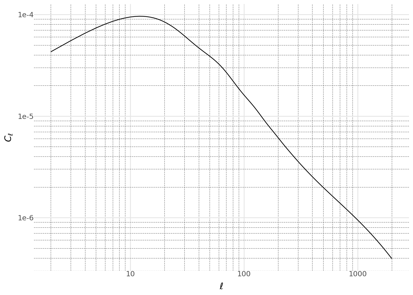
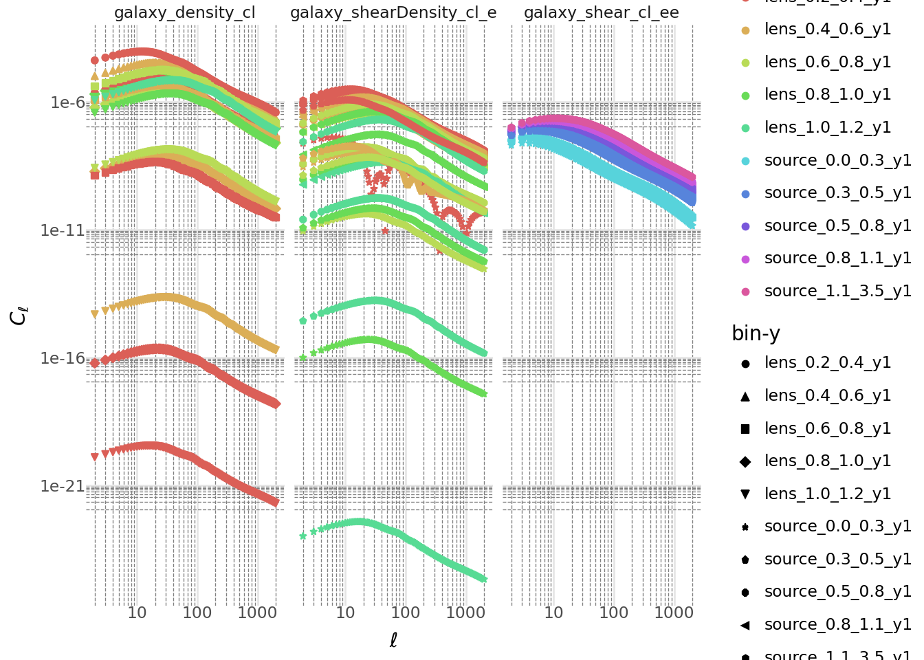
The plot above illustrates the first pair of bins. To complete the analysis, we can generate the two-point statistics for all bin pairs.
Code
two_point_pd_list = []
for two_point, meta in zip(all_two_point_functions, all_two_point_cells):
    two_point_pd_list.append(
        pd.DataFrame(
            {
                "ell": two_point.ells,
                "Cell": np.abs(two_point.compute_theory_vector(tools)),
                "bin-x": meta.XY.x.bin_name,
                "bin-y": meta.XY.y.bin_name,
                "measurement": meta.get_sacc_name(),
            }
        )
    )

data = pd.concat(two_point_pd_list)

(
    ggplot(data, aes("ell", "Cell", color="bin-x", shape="bin-y"))
    + geom_point()
    + labs(x=r"$\ell$", y=r"$C_\ell$")
    + scale_x_log10()
    + scale_y_log10()
    + facet_wrap("measurement")
    + doc_theme()
)