Using Firecrown Factories to Initialize Two-Point Objects

version 1.14.2

def doc_theme():
    return theme_minimal() + theme(
        panel_grid_minor=element_line(color="gray", linetype="--"),
    )

Purpose of this Document

This tutorial explains how the TwoPointFactory automates the construction of TwoPoint likelihood objects in Firecrown. It leverages Firecrown’s hierarchical metadata framework, described in Two-Point Framework, to translate abstract metadata and input data into fully configured measurement pipelines—ensuring consistency and minimizing redundancy across analyses.

Framework Hierarchy Overview

Firecrown’s two-point framework organizes metadata into four layers:

1. Bin Descriptors (e.g., InferredGalaxyZDist)
   • Define properties of individual observables (e.g., redshift distributions, tracer types).
     
   • Shared across components to enforce configuration consistency by construction.
2. Bin Pairs (TwoPointXY)
   • Represent cross-correlations between two bins (e.g., galaxy lensing × galaxy clustering).
     
   • Ensure consistency of paired bin definitions (e.g., redshift ranges, tracer compatibility).
3. Data Layouts
   • Describe the measurement structure:
     • TwoPointHarmonic: for harmonic-space statistics (e.g., \(C(\ell)\)).
       
     • TwoPointReal: for real-space statistics (e.g., \(\xi(\theta)\)).
       
   • Contain only metadata (no observational data), making them reusable for theory comparisons or forecasting.
4. Measurement Containers (TwoPointMeasurement)
   • Combine a data layout with observed or simulated data.

Role of the TwoPointFactory

The TwoPointFactory serves as the interface between data layout definitions and the construction of TwoPoint objects. It handles:

1. Parsing layout metadata from:
   • Manually defined configurations (e.g., YAML descriptors).
     
   • Automated pipelines (Two-Point Generators).
     
   • SACC files, with or without embedded data.
2. Building TwoPoint objects that:
   • Map tracer definitions (e.g., galaxy samples, lens bins) to measurement configurations.
     
   • Establish the link between theory predictions and data layout.
     
   • Optionally incorporate observational data, producing the associated DataVector.

The tutorials InferredGalaxyZDist, InferredGalaxyZDist Generators, and InferredGalaxyZDist Serialization describe how to construct and serialize redshift distribution objects. Here, we focus specifically on extracting layout and redshift information from a SACC object to support the use of TwoPointFactory.

SACC Workflows

• Full SACC extraction: Loads both metadata and data, yielding a fully configured TwoPoint object.
  
• Partial SACC extraction (deprecated):
  • Loads only data indices, requiring manual invocation of TwoPoint.read to attach data.
    
  • Lacks TypeSource information, preventing automated source configuration.

Working with SACC Objects

A SACC object provides all components needed for a statistical analysis in Firecrown:

• Metadata: Layout, data types, binning, tracer names.
• Calibration data: Redshift distributions \(\mathrm{d}n/\mathrm{d}z\) for each bin.
• Data: Measurements (e.g., power spectra).
• Covariance: Uncertainties and correlations.

Firecrown supports two workflows: the recommended full extraction approach, and a legacy indices-only approach, now deprecated.

Recommended: Full Metadata + Data Extraction

In the current interface, Firecrown extracts everything from a SACC object — layout, calibration, and measurements. These are passed directly to constructors that build ready-to-use likelihoods.

from firecrown.data_functions import (
    extract_all_real_data,
    check_two_point_consistence_real,
)
from firecrown.likelihood.factories import load_sacc_data

sacc_data = load_sacc_data("../examples/des_y1_3x2pt/sacc_data.hdf5")

two_point_reals = extract_all_real_data(sacc_data)
check_two_point_consistence_real(two_point_reals)

Use a factory to build the TwoPoint objects in the ready state:

from firecrown.likelihood.two_point import TwoPoint, TwoPointFactory
from firecrown.utils import (
    base_model_from_yaml,
    ClIntegrationMethod,
    ClIntegrationOptions,
    ClLimberMethod,
)

two_point_yaml = """
correlation_space: real
weak_lensing_factories:
  - type_source: default
    per_bin_systematics:
    - type: MultiplicativeShearBiasFactory
    - type: PhotoZShiftFactory
    global_systematics:
    - type: LinearAlignmentSystematicFactory
      alphag: 1.0
number_counts_factories:
  - type_source: default
    per_bin_systematics:
    - type: PhotoZShiftFactory
    global_systematics: []
"""

tp_factory = base_model_from_yaml(TwoPointFactory, two_point_yaml)
two_points_ready = TwoPoint.from_measurement(two_point_reals, tp_factory)

Create a Likelihood object in the ready state using the covariance matrix:

from firecrown.likelihood.gaussian import ConstGaussian

likelihood_ready = ConstGaussian.create_ready(
    two_points_ready, sacc_data.covariance.dense
)

Deprecated: Indices-Only Extraction

This approach was used in Firecrown \(\leq 1.7\). Users needed to know the structure of the SACC file a priori and create TwoPoint objects manually.

To reduce this burden, Firecrown introduced a helper to extract tracer pairs and data types from a SACC file:

from firecrown.metadata_functions import extract_all_real_metadata_indices
from firecrown.likelihood.factories import load_sacc_data

# Load the SACC file
sacc_data = load_sacc_data("../examples/des_y1_3x2pt/sacc_data.hdf5")
# Extract all metadata indices
all_meta = extract_all_real_metadata_indices(sacc_data)

You can inspect the extracted metadata layout:

import yaml
from IPython.display import Markdown

all_meta_prune = [
    {
        "data_type": meta["data_type"],
        "tracer1": str(meta["tracer_names"].name1),
        "tracer2": str(meta["tracer_names"].name2),
    }
    for meta in all_meta
]

all_meta_yaml = yaml.safe_dump(all_meta_prune[::4], default_flow_style=False)
Markdown(f"```yaml\n{all_meta_yaml}\n```")

- data_type: galaxy_density_xi
  tracer1: lens0
  tracer2: lens0
- data_type: galaxy_density_xi
  tracer1: lens4
  tracer2: lens4
- data_type: galaxy_shearDensity_xi_t
  tracer1: lens0
  tracer2: src3
- data_type: galaxy_shearDensity_xi_t
  tracer1: lens1
  tracer2: src3
- data_type: galaxy_shearDensity_xi_t
  tracer1: lens2
  tracer2: src3
- data_type: galaxy_shearDensity_xi_t
  tracer1: lens3
  tracer2: src3
- data_type: galaxy_shearDensity_xi_t
  tracer1: lens4
  tracer2: src3
- data_type: galaxy_shear_xi_minus
  tracer1: src0
  tracer2: src3
- data_type: galaxy_shear_xi_minus
  tracer1: src2
  tracer2: src2
- data_type: galaxy_shear_xi_plus
  tracer1: src0
  tracer2: src1
- data_type: galaxy_shear_xi_plus
  tracer1: src1
  tracer2: src2
- data_type: galaxy_shear_xi_plus
  tracer1: src3
  tracer2: src3

Construct the TwoPoint objects using the extracted layout and the factory:

tp_factory = base_model_from_yaml(TwoPointFactory, two_point_yaml)
two_point_list = TwoPoint.from_metadata_index(all_meta, tp_factory)

At this stage, the TwoPoint objects contain only structural metadata (e.g., tracer combinations, data types). They are not yet in the ready state, as no metadata or measurement data has been attached. To complete the construction, you must call the Statistic.read method on each object. Alternatively, if the TwoPoint objects are part of a Likelihood instance, calling its Likelihood.read method will internally propagate to each contained statistic:

likelihood = ConstGaussian(two_point_list)
likelihood.read(sacc_data)

Each TwoPoint object is a subclass of Statistic, and the Likelihood.read method delegates to Statistic.read for each of its components.

Note: This indices-only method is deprecated and kept for compatibility with older code. For new projects, prefer the full extraction interface above.

Comparing Results

We now verify that both approaches—constructing the likelihood in two phases (metadata-only) and directly in the ready state—produce identical results.

First, we extract the required parameter sets for both likelihoods:

from firecrown.parameters import ParamsMap

req_params = likelihood.required_parameters()
req_params_ready = likelihood_ready.required_parameters()

assert req_params_ready == req_params

default_values = req_params.get_default_values()
params = ParamsMap(default_values)

Both likelihoods depend on the same parameter set. The default values used are:

import yaml
from IPython.display import Markdown

default_values_yaml = yaml.dump(default_values, default_flow_style=False)
Markdown(f"```yaml\n{default_values_yaml}\n```")

alphaz: 0.0
ia_bias: 0.5
lens0_bias: 1.5
lens0_delta_z: 0.0
lens1_bias: 1.5
lens1_delta_z: 0.0
lens2_bias: 1.5
lens2_delta_z: 0.0
lens3_bias: 1.5
lens3_delta_z: 0.0
lens4_bias: 1.5
lens4_delta_z: 0.0
src0_delta_z: 0.0
src0_mult_bias: 1.0
src1_delta_z: 0.0
src1_mult_bias: 1.0
src2_delta_z: 0.0
src2_mult_bias: 1.0
src3_delta_z: 0.0
src3_mult_bias: 1.0
z_piv: 0.5

Next, we prepare both likelihoods with the same model setup and parameters:

from firecrown.modeling_tools import ModelingTools
from firecrown.ccl_factory import CCLFactory
from firecrown.updatable import get_default_params_map

tools = ModelingTools(ccl_factory=CCLFactory(require_nonlinear_pk=True))
params = get_default_params_map(tools, likelihood)

tools.update(params)
tools.prepare()

likelihood.update(params)
likelihood_ready.update(params)

Finally, we compute and compare the log-likelihood values from both construction methods:

print(f"Loglike (metadata-only): {likelihood.compute_loglike(tools)}")
print(f"Loglike (ready state):   {likelihood_ready.compute_loglike(tools)}")

Loglike (metadata-only): -2742.739024737394
Loglike (ready state):   -2742.739024737394

Both values should match exactly, confirming that the two construction methods are consistent.

Filtering Data: Scale-cuts

Real analyses use only a subset of the measured two-points statistics, where the utilized data is typically limited my the accuracy of the models used to fit the data. It is then useful to define the physical scales (corresponding to the data) that should be analyzed in a given likelihood evaluation of two-point statistics. Firecrown can implement this feature though its factories, notably by defining a TwoPointBinFilterCollection object. This object is a collection of TwoPointBinFilter objects, which define the valid data analysis range for a given combination of two-point tracers. For instance, we can define the filtered range of galaxy clustering auto-correlations as follows:

from firecrown.data_functions import TwoPointBinFilterCollection, TwoPointBinFilter
from firecrown.metadata_types import Galaxies
from firecrown.utils import base_model_to_yaml

tp_collection = TwoPointBinFilterCollection(
    filters=[
        TwoPointBinFilter.from_args(
            name1=f"lens{i}",
            measurement1=Galaxies.COUNTS,
            name2=f"lens{i}",
            measurement2=Galaxies.COUNTS,
            lower=2,
            upper=300,
        )
        for i in range(5)
    ],
    require_filter_for_all=True,
    allow_empty=True,
)
Markdown(f"```yaml\n{base_model_to_yaml(tp_collection)}\n```")

require_filter_for_all: true
allow_empty: true
filters:
- spec:
  - name: lens0
    measurement: {subject: Galaxies, property: COUNTS}
  - name: lens0
    measurement: {subject: Galaxies, property: COUNTS}
  interval: [2.0, 300.0]
  method: support
- spec:
  - name: lens1
    measurement: {subject: Galaxies, property: COUNTS}
  - name: lens1
    measurement: {subject: Galaxies, property: COUNTS}
  interval: [2.0, 300.0]
  method: support
- spec:
  - name: lens2
    measurement: {subject: Galaxies, property: COUNTS}
  - name: lens2
    measurement: {subject: Galaxies, property: COUNTS}
  interval: [2.0, 300.0]
  method: support
- spec:
  - name: lens3
    measurement: {subject: Galaxies, property: COUNTS}
  - name: lens3
    measurement: {subject: Galaxies, property: COUNTS}
  interval: [2.0, 300.0]
  method: support
- spec:
  - name: lens4
    measurement: {subject: Galaxies, property: COUNTS}
  - name: lens4
    measurement: {subject: Galaxies, property: COUNTS}
  interval: [2.0, 300.0]
  method: support

Equivalently, we may reduce the complexity of the code slightly and specify the use of auto-correlations only:

tp_collection = TwoPointBinFilterCollection(
                filters=[
                    TwoPointBinFilter.from_args_auto(
                        name=f"lens{i}",
                        measurement=Galaxies.COUNTS,
                        lower=2,
                        upper=300,
                    )
                    for i in range(5)
                ],
                require_filter_for_all=True,
                allow_empty=True,
)
Markdown(f"```yaml\n{base_model_to_yaml(tp_collection)}\n```")

require_filter_for_all: true
allow_empty: true
filters:
- spec:
  - name: lens0
    measurement: {subject: Galaxies, property: COUNTS}
  interval: [2.0, 300.0]
  method: support
- spec:
  - name: lens1
    measurement: {subject: Galaxies, property: COUNTS}
  interval: [2.0, 300.0]
  method: support
- spec:
  - name: lens2
    measurement: {subject: Galaxies, property: COUNTS}
  interval: [2.0, 300.0]
  method: support
- spec:
  - name: lens3
    measurement: {subject: Galaxies, property: COUNTS}
  interval: [2.0, 300.0]
  method: support
- spec:
  - name: lens4
    measurement: {subject: Galaxies, property: COUNTS}
  interval: [2.0, 300.0]
  method: support

One may alternatively define the tracers directly (instead of from arguments) as TwoPointTracerSpec objects.

A TwoPointExperiment object is able to keep track of the relevant Factory instances to generate the two-point configurations of the analysis (either in configuration or harmonic space) and the scale-cut/data filtering choices to evaluate a defined likelihood. The interpretation of the filtered lower and upper limits of the data depend on the definition of the TwoPointExperiment factories in either configuration or harmonic space.

With this formalism, we are able to evaluate the likelihood exactly as the previous section by defining filters to be very wide. Alternatively, by setting a restrictively small filtered range, we can remove data from the analysis and do so in the example below by filtering-out all galaxy clustering data.

from firecrown.likelihood.factories import (
    DataSourceSacc,
    TwoPointCorrelationSpace,
    TwoPointExperiment,
    TwoPointFactory,
)

tpf = base_model_from_yaml(TwoPointFactory, two_point_yaml)

two_point_experiment = TwoPointExperiment(
    two_point_factory=tpf,
    data_source=DataSourceSacc(
        sacc_data_file="../examples/des_y1_3x2pt/sacc_data.hdf5",
        filters=TwoPointBinFilterCollection(
            require_filter_for_all=False,
            allow_empty=True,
            filters=[
                TwoPointBinFilter.from_args_auto(
                    name=f"lens{i}",
                    measurement=Galaxies.COUNTS,
                    lower=0.5,
                    upper=300,
                )
                for i in range(5)
            ],
        ),
    ),
)

two_point_experiment_filtered = TwoPointExperiment(
    two_point_factory=tpf,
    data_source=DataSourceSacc(
        sacc_data_file="../examples/des_y1_3x2pt/sacc_data.hdf5",
        filters=TwoPointBinFilterCollection(
            require_filter_for_all=False,
            allow_empty=True,
            filters=[
                TwoPointBinFilter.from_args_auto(
                    name=f"lens{i}",
                    measurement=Galaxies.COUNTS,
                    lower=2999,
                    upper=3000,
                )
                for i in range(5)
            ],
        ),
    ),
)

The TwoPointExperiment objects can also be used to create likelihoods in the ready state. Additionally, they can be serialized into a yaml file, making it easier to share specific analysis choices with other users and collaborators.

The yaml below shows the first experiment.

Markdown(f"```yaml\n{base_model_to_yaml(two_point_experiment)}\n```")

two_point_factory:
  correlation_space: real
  weak_lensing_factories:
  - type_source: default
    per_bin_systematics:
    - {type: MultiplicativeShearBiasFactory}
    - {type: PhotoZShiftFactory}
    global_systematics:
    - {type: LinearAlignmentSystematicFactory, alphag: 1.0}
  number_counts_factories:
  - type_source: default
    per_bin_systematics:
    - {type: PhotoZShiftFactory}
    global_systematics: []
    include_rsd: false
  cmb_factories: []
  int_options: null
data_source:
  sacc_data_file: ../examples/des_y1_3x2pt/sacc_data.hdf5
  filters:
    require_filter_for_all: false
    allow_empty: true
    filters:
    - spec:
      - name: lens0
        measurement: {subject: Galaxies, property: COUNTS}
      interval: [0.5, 300.0]
      method: support
    - spec:
      - name: lens1
        measurement: {subject: Galaxies, property: COUNTS}
      interval: [0.5, 300.0]
      method: support
    - spec:
      - name: lens2
        measurement: {subject: Galaxies, property: COUNTS}
      interval: [0.5, 300.0]
      method: support
    - spec:
      - name: lens3
        measurement: {subject: Galaxies, property: COUNTS}
      interval: [0.5, 300.0]
      method: support
    - spec:
      - name: lens4
        measurement: {subject: Galaxies, property: COUNTS}
      interval: [0.5, 300.0]
      method: support
ccl_factory: {require_nonlinear_pk: false, amplitude_parameter: sigma8, mass_split: normal,
  num_neutrino_masses: null, creation_mode: default, pure_ccl_transfer_function: boltzmann_camb,
  use_camb_hm_sampling: false, allow_multiple_camb_instances: false, camb_extra_params: null,
  ccl_spline_params: null, parameter_prefix: null}

The yaml below shows the second experiment.

Markdown(f"```yaml\n{base_model_to_yaml(two_point_experiment_filtered)}\n```")

two_point_factory:
  correlation_space: real
  weak_lensing_factories:
  - type_source: default
    per_bin_systematics:
    - {type: MultiplicativeShearBiasFactory}
    - {type: PhotoZShiftFactory}
    global_systematics:
    - {type: LinearAlignmentSystematicFactory, alphag: 1.0}
  number_counts_factories:
  - type_source: default
    per_bin_systematics:
    - {type: PhotoZShiftFactory}
    global_systematics: []
    include_rsd: false
  cmb_factories: []
  int_options: null
data_source:
  sacc_data_file: ../examples/des_y1_3x2pt/sacc_data.hdf5
  filters:
    require_filter_for_all: false
    allow_empty: true
    filters:
    - spec:
      - name: lens0
        measurement: {subject: Galaxies, property: COUNTS}
      interval: [2999.0, 3000.0]
      method: support
    - spec:
      - name: lens1
        measurement: {subject: Galaxies, property: COUNTS}
      interval: [2999.0, 3000.0]
      method: support
    - spec:
      - name: lens2
        measurement: {subject: Galaxies, property: COUNTS}
      interval: [2999.0, 3000.0]
      method: support
    - spec:
      - name: lens3
        measurement: {subject: Galaxies, property: COUNTS}
      interval: [2999.0, 3000.0]
      method: support
    - spec:
      - name: lens4
        measurement: {subject: Galaxies, property: COUNTS}
      interval: [2999.0, 3000.0]
      method: support
ccl_factory: {require_nonlinear_pk: false, amplitude_parameter: sigma8, mass_split: normal,
  num_neutrino_masses: null, creation_mode: default, pure_ccl_transfer_function: boltzmann_camb,
  use_camb_hm_sampling: false, allow_multiple_camb_instances: false, camb_extra_params: null,
  ccl_spline_params: null, parameter_prefix: null}

Next, we can create likelihoods from the TwoPointExperiment objects and compare the loglike values.

likelihood_tpe = two_point_experiment.make_likelihood()

params = get_default_params_map(tools, likelihood_tpe)

tools = ModelingTools()
tools.update(params)
tools.prepare()
likelihood_tpe.update(params)

likelihood_tpe_filtered = two_point_experiment_filtered.make_likelihood()

params = get_default_params_map(tools, likelihood_tpe_filtered)

tools = ModelingTools()
tools.update(params)
tools.prepare()
likelihood_tpe_filtered.update(params)

print(f"Loglike from metadata only: {likelihood.compute_loglike(tools)}")
print(f"Loglike from ready state: {likelihood_ready.compute_loglike(tools)}")
print(f"Loglike from TwoPointExperiment: {likelihood_tpe.compute_loglike(tools)}")
print(f"Loglike from filtered TwoPointExperiment: {likelihood_tpe_filtered.compute_loglike(tools)}")

Loglike from metadata only: -2742.739024737394
Loglike from ready state: -2742.739024737394
Loglike from TwoPointExperiment: -2742.739024737394
Loglike from filtered TwoPointExperiment: -2579.948781562013

Controlling Integration

TwoPointFactory objects can include integration options, allowing control over how two-point functions are computed.
The example below shows how to create a TwoPointFactory with integration options that reproduce the default behavior.
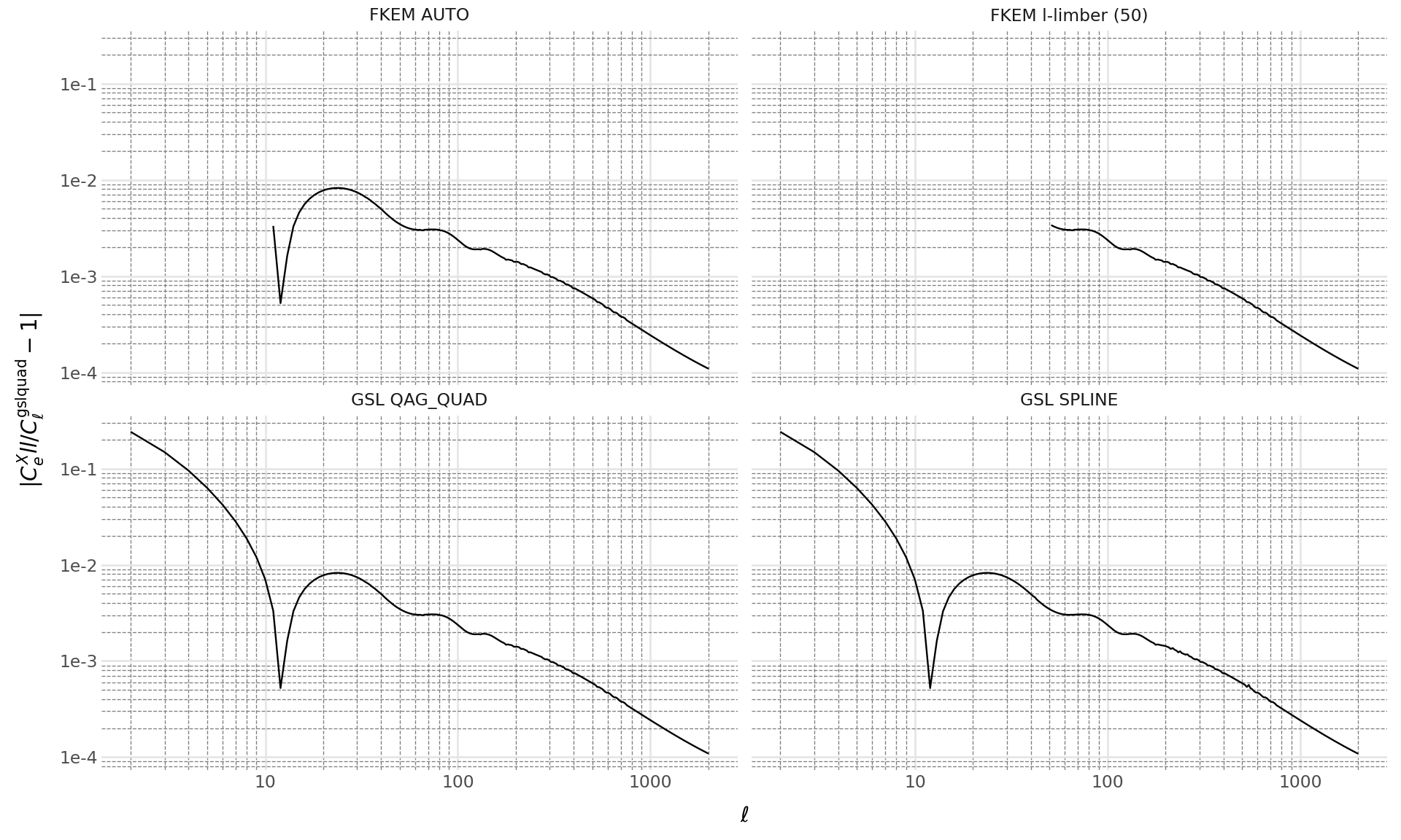
We also create additional TwoPointFactory objects with alternative integration configurations: ClIntegrationMethod.LIMBER with ClLimberMethod.GSL_SPLINE, ClIntegrationMethod.FKEM_AUTO, and ClIntegrationMethod.FKEM_L_LIMBER.

The lens and source redshift bin collections used for the computations are imported from the firecrown.generators.inferred_galaxy_zdist module:
LSST_Y1_LENS_HARMONIC_BIN_COLLECTION and LSST_Y1_SOURCE_HARMONIC_BIN_COLLECTION.

import numpy as np
from firecrown.metadata_functions import make_all_photoz_bin_combinations
from firecrown.metadata_types import TwoPointHarmonic
from firecrown.generators.inferred_galaxy_zdist import (
    LSST_Y1_LENS_HARMONIC_BIN_COLLECTION,
    LSST_Y1_SOURCE_HARMONIC_BIN_COLLECTION,
)

count_bins = LSST_Y1_LENS_HARMONIC_BIN_COLLECTION.generate()
shear_bins = LSST_Y1_SOURCE_HARMONIC_BIN_COLLECTION.generate()
all_y1_bins = count_bins[:1] + shear_bins[:1]

all_two_point_xy = make_all_photoz_bin_combinations(all_y1_bins)
ells = np.unique(
    np.concatenate((np.arange(2, 120), np.geomspace(120, 2000, 128)))
).astype(int)
all_two_point_cells = [TwoPointHarmonic(XY=xy, ells=ells) for xy in all_two_point_xy]

tpf_gsl_quad = TwoPointFactory(
    correlation_space=TwoPointCorrelationSpace.HARMONIC,
    weak_lensing_factories=tpf.weak_lensing_factories,
    number_counts_factories=tpf.number_counts_factories,
    int_options=ClIntegrationOptions(
        method=ClIntegrationMethod.LIMBER, limber_method=ClLimberMethod.GSL_QAG_QUAD
    ),
)

tpf_gsl_spline = TwoPointFactory(
    correlation_space=TwoPointCorrelationSpace.HARMONIC,
    weak_lensing_factories=tpf.weak_lensing_factories,
    number_counts_factories=tpf.number_counts_factories,
    int_options=ClIntegrationOptions(
        method=ClIntegrationMethod.LIMBER, limber_method=ClLimberMethod.GSL_SPLINE
    ),
)

tpf_fkem_auto = TwoPointFactory(
    correlation_space=TwoPointCorrelationSpace.HARMONIC,
    weak_lensing_factories=tpf.weak_lensing_factories,
    number_counts_factories=tpf.number_counts_factories,
    int_options=ClIntegrationOptions(
        method=ClIntegrationMethod.FKEM_AUTO, limber_method=ClLimberMethod.GSL_QAG_QUAD
    ),
)

tpf_fkem_l_limber = TwoPointFactory(
    correlation_space=TwoPointCorrelationSpace.HARMONIC,
    weak_lensing_factories=tpf.weak_lensing_factories,
    number_counts_factories=tpf.number_counts_factories,
    int_options=ClIntegrationOptions(
        method=ClIntegrationMethod.FKEM_L_LIMBER,
        limber_method=ClLimberMethod.GSL_QAG_QUAD,
        l_limber=50,
    ),
)

tpf_fkem_l_limber_max = TwoPointFactory(
    correlation_space=TwoPointCorrelationSpace.HARMONIC,
    weak_lensing_factories=tpf.weak_lensing_factories,
    number_counts_factories=tpf.number_counts_factories,
    int_options=ClIntegrationOptions(
        method=ClIntegrationMethod.FKEM_L_LIMBER,
        limber_method=ClLimberMethod.GSL_QAG_QUAD,
        l_limber=2100,
    ),
)

two_points_gsl_quad = tpf_gsl_quad.from_metadata(all_two_point_cells)
two_points_gsl_spline = tpf_gsl_spline.from_metadata(all_two_point_cells)
two_points_fkem_auto = tpf_fkem_auto.from_metadata(all_two_point_cells)
two_points_fkem_l_limber = tpf_fkem_l_limber.from_metadata(all_two_point_cells)
two_points_fkem_l_limber_max = tpf_fkem_l_limber_max.from_metadata(all_two_point_cells)

Now we plot the relative differences between each integration method and the most accurate (FKEM applied to all ells), highlighting the impact of different integration choices on the two-point functions.

from plotnine import *  # bad form in programs, but seems OK for plotnine
import pandas as pd

two_point0_gsl_quad = two_points_gsl_quad[0]
two_point0_gsl_spline = two_points_gsl_spline[0]
two_point0_fkem_auto = two_points_fkem_auto[0]
two_point0_fkem_l_limber = two_points_fkem_l_limber[0]
two_point0_fkem_l_limber_max = two_points_fkem_l_limber_max[0]
meta0 = all_two_point_cells[0]

two_point0_gsl_quad.update(get_default_params_map(two_point0_gsl_quad))
two_point0_gsl_spline.update(get_default_params_map(two_point0_gsl_spline))
two_point0_fkem_auto.update(get_default_params_map(two_point0_fkem_auto))
two_point0_fkem_l_limber.update(get_default_params_map(two_point0_fkem_l_limber))
two_point0_fkem_l_limber_max.update(
    get_default_params_map(two_point0_fkem_l_limber_max)
)

tv0_gsl_quad = two_point0_gsl_quad.compute_theory_vector(tools)
tv0_gsl_spline = two_point0_gsl_spline.compute_theory_vector(tools)
tv0_fkem_auto = two_point0_fkem_auto.compute_theory_vector(tools)
tv0_fkem_l_limber = two_point0_fkem_l_limber.compute_theory_vector(tools)
tv0_fkem_l_limber_max = two_point0_fkem_l_limber_max.compute_theory_vector(tools)

tmp = np.abs(tv0_gsl_spline / tv0_fkem_l_limber_max - 1.0)
data_gsl_spline = pd.DataFrame(
    {
        "ell": two_point0_gsl_spline.ells[tmp > 0.0],
        "rel-diff": tmp[tmp > 0.0],
        "bin-x": meta0.XY.x.bin_name,
        "bin-y": meta0.XY.y.bin_name,
        "measurement": meta0.get_sacc_name(),
        "integration": "GSL SPLINE",
    }
)

tmp = np.abs(tv0_gsl_quad / tv0_fkem_l_limber_max - 1.0)
data_gsl_quad = pd.DataFrame(
    {
        "ell": two_point0_gsl_quad.ells[tmp > 0.0],
        "rel-diff": tmp[tmp > 0.0],
        "bin-x": meta0.XY.x.bin_name,
        "bin-y": meta0.XY.y.bin_name,
        "measurement": meta0.get_sacc_name(),
        "integration": "GSL QAG_QUAD",
    }
)

tmp = np.abs(tv0_fkem_auto / tv0_fkem_l_limber_max - 1.0)
data_fkem_auto = pd.DataFrame(
    {
        "ell": two_point0_fkem_auto.ells[tmp > 0.0],
        "rel-diff": tmp[tmp > 0.0],
        "bin-x": meta0.XY.x.bin_name,
        "bin-y": meta0.XY.y.bin_name,
        "measurement": meta0.get_sacc_name(),
        "integration": "FKEM AUTO",
    }
)

tmp = np.abs(tv0_fkem_l_limber / tv0_fkem_l_limber_max - 1.0)
data_fkem_l_limber = pd.DataFrame(
    {
        "ell": two_point0_fkem_l_limber.ells[tmp > 0.0],
        "rel-diff": tmp[tmp > 0.0],
        "bin-x": meta0.XY.x.bin_name,
        "bin-y": meta0.XY.y.bin_name,
        "measurement": meta0.get_sacc_name(),
        "integration": "FKEM l-limber (50)",
    }
)

data = pd.concat([data_gsl_spline, data_gsl_quad, data_fkem_auto, data_fkem_l_limber])

# Now we can generate the plot.
(
    ggplot(data, aes("ell", "rel-diff"))
    + geom_line()
    + labs(x=r"$\ell$", y=r"$|C^X_ell/C^\mathrm{gsl quad}_\ell - 1|$")
    + scale_x_log10()
    + scale_y_log10()
    + doc_theme()
    + facet_wrap("integration")
    + theme(figure_size=(10, 6))
)

/home/docs/checkouts/readthedocs.org/user_builds/firecrown/conda/v1.14.2/lib/python3.14/site-packages/pyccl/errors.py:22: CCLWarning: Nchi must be a positive integer. Setting to match tracer with large chi samples x 2.
/home/docs/checkouts/readthedocs.org/user_builds/firecrown/conda/v1.14.2/lib/python3.14/site-packages/pyccl/errors.py:22: CCLWarning: chi_min must be greater than zero.Setting to default 1e-6 Mpc.

Figure 1: Relative difference to default behavior