Factory Basics: Constructing TwoPoint Objects

Version ?env:FIRECROWN_VERSION

def doc_theme():
    return theme_minimal() + theme(
        panel_grid_minor=element_line(color="gray", linetype="--"),
    )

Purpose of this Document

This tutorial explains how to use the TwoPointFactory to construct TwoPoint objects from metadata and optional data. This is the core mechanism for building likelihood objects, regardless of whether your metadata came from generators or SACC files.

For conceptual background, see Two-Point Framework.

The Role of TwoPointFactory

The TwoPointFactory automates the construction of TwoPoint likelihood objects. It:

1. Inspects metadata to determine what types of measurements are involved
2. Delegates to source factories (e.g., WeakLensingFactory, NumberCountsFactory) based on measurement types
3. Applies modeling choices including systematics and nuisance parameters
4. Produces ready-to-use TwoPoint objects that can compute theory predictions or evaluate likelihoods

Input: Metadata ± Data

The factory accepts either:

• Layout only (TwoPointHarmonic or TwoPointReal) → produces theory-only TwoPoint objects
• Measurement (TwoPointMeasurement) → produces TwoPoint objects with both data and theory

The metadata can come from two sources:

1. Generated (Two-Point Generators): Programmatically created using Firecrown’s generators
2. Extracted (Loading SACC Data): Read from existing SACC files

Regardless of source, the factory treats the metadata identically.

Output: TwoPoint Objects

Each produced TwoPoint object: - Contains all modeling assumptions (systematics, bias models, etc.) - Can compute theoretical predictions via compute_theory_vector() - If created from measurement data, can contribute to likelihood evaluation - Is a subclass of Statistic and can be combined into a Likelihood

Source Factory Mapping

The TwoPointFactory automatically maps measurement types to appropriate source factories:

• Galaxies.COUNTS → NumberCountsFactory
• Galaxies.SHEAR_E, Galaxies.SHEAR_T, etc. → WeakLensingFactory

Multiple TypeSource Support

The factory can hold multiple instances of the same source factory type, each associated with a different TypeSource. This enables distinct modeling choices for subpopulations:

# Example: Different systematics for red vs. blue galaxies
factory = TwoPointFactory(
    correlation_space=TwoPointCorrelationSpace.HARMONIC,
    number_counts_factories=[
        NumberCountsFactory(type_source="red", ...),
        NumberCountsFactory(type_source="blue", ...),
    ]
)

By default, both bins and factories use TypeSource.DEFAULT, so simple analyses don’t need to worry about this feature.

Metadata Structure Overview

Before using the factory, it’s helpful to understand Firecrown’s four-layer metadata hierarchy:

1. Bin Descriptors (e.g., InferredGalaxyZDist)
   • Properties of individual observables (redshift distributions, tracer types)
   • Shared across components for consistency
2. Bin Pairs (TwoPointXY)
   • Cross-correlations between two bins
   • Ensures paired bin compatibility
3. Data Layouts (TwoPointHarmonic or TwoPointReal)
   • Measurement structure: harmonic space (\(C_\ell\)) or real space (\(\xi(\theta)\))
   • Metadata only — no observational data
4. Measurement Containers (TwoPointMeasurement)
   • Combines layout with observed/simulated data

See Two-Point Framework for detailed explanation.

Where Metadata Comes From

There are two primary workflows for obtaining the metadata that the factory needs:

1. Generate from Scratch

Two-Point Generators shows how to: - Create InferredGalaxyZDist bins programmatically - Generate LSST-SRD redshift distributions - Define systematics factories - Build metadata layouts

Use this when creating forecasts or simulations.

2. Extract from SACC Files

Loading SACC Data shows how to: - Extract metadata and data from SACC files - Use full extraction (recommended) or legacy indices-only approach - Validate extracted data consistency

Use this when working with real observations or pre-existing data files.

Complete Example: Generated Metadata

This example shows the full workflow starting from generated metadata. For details on generating the LSST Year 1 bins and metadata, see Two-Point Generators. In this example we use the 3x2pt bin pair selection logic from Bin Pair Selectors.

Step 1: Generate Metadata

import numpy as np
from firecrown.generators import (
    LSST_Y1_LENS_HARMONIC_BIN_COLLECTION,
    LSST_Y1_SOURCE_HARMONIC_BIN_COLLECTION,
)
from firecrown.metadata_functions import make_binned_two_point_filtered
from firecrown.metadata_types import TwoPointHarmonic, ThreeTwoBinPairSelector

# Generate LSST Y1 bins
count_bins = LSST_Y1_LENS_HARMONIC_BIN_COLLECTION.generate()
shear_bins = LSST_Y1_SOURCE_HARMONIC_BIN_COLLECTION.generate()
all_y1_bins = count_bins + shear_bins

# Create two-point combinations using 3x2pt logic
bin_pair_selector = ThreeTwoBinPairSelector(
    lens_dist=1, source_dist=1, source_lens_dist=5
)
all_two_point_xy = make_binned_two_point_filtered(all_y1_bins, bin_pair_selector)
ells = np.unique(np.geomspace(2, 2000, 128).astype(int))
all_two_point_cells = [TwoPointHarmonic(XY=xy, ells=ells) for xy in all_two_point_xy]

Step 2: Define Systematics Factories

import firecrown.likelihood.weak_lensing as wl
import firecrown.likelihood.number_counts as nc
from firecrown.likelihood.weak_lensing import PhotoZShiftFactory

# WeakLensing systematics
ia_systematic = wl.LinearAlignmentSystematicFactory()
wl_photoz = PhotoZShiftFactory()
wl_mult_bias = wl.MultiplicativeShearBiasFactory()

wlf = wl.WeakLensingFactory(
    per_bin_systematics=[wl_mult_bias, wl_photoz],
    global_systematics=[ia_systematic],
)

# NumberCounts systematics
nc_photoz = PhotoZShiftFactory()
ncf = nc.NumberCountsFactory(
    per_bin_systematics=[nc_photoz],
    global_systematics=[],
)

Systematics factories can be serialized for reuse:

from firecrown.utils import base_model_to_yaml

wl_yaml = base_model_to_yaml(wlf)
nc_yaml = base_model_to_yaml(ncf)

Step 3: Construct TwoPoint Objects

from firecrown.likelihood import TwoPoint, TwoPointFactory
from firecrown.metadata_types import TwoPointCorrelationSpace

all_two_point_functions = TwoPoint.from_metadata(
    metadata_seq=all_two_point_cells,
    tp_factory=TwoPointFactory(
        correlation_space=TwoPointCorrelationSpace.HARMONIC,
        weak_lensing_factories=[wlf],
        number_counts_factories=[ncf],
    ),
)

Step 4: Setup and Compute Predictions

from firecrown.modeling_tools import ModelingTools
from firecrown.modeling_tools import CCLFactory
from firecrown.updatable import get_default_params
from firecrown.updatable import ParamsMap

# Setup modeling tools and parameters
tools = ModelingTools(ccl_factory=CCLFactory(require_nonlinear_pk=True))
default_values = get_default_params(tools, all_two_point_functions)
params = ParamsMap(default_values)

# Prepare for computation
tools.update(params)
tools.prepare()
all_two_point_functions.update(params)

Compute theory predictions:

two_point0 = all_two_point_functions[0]
meta0 = all_two_point_cells[0]
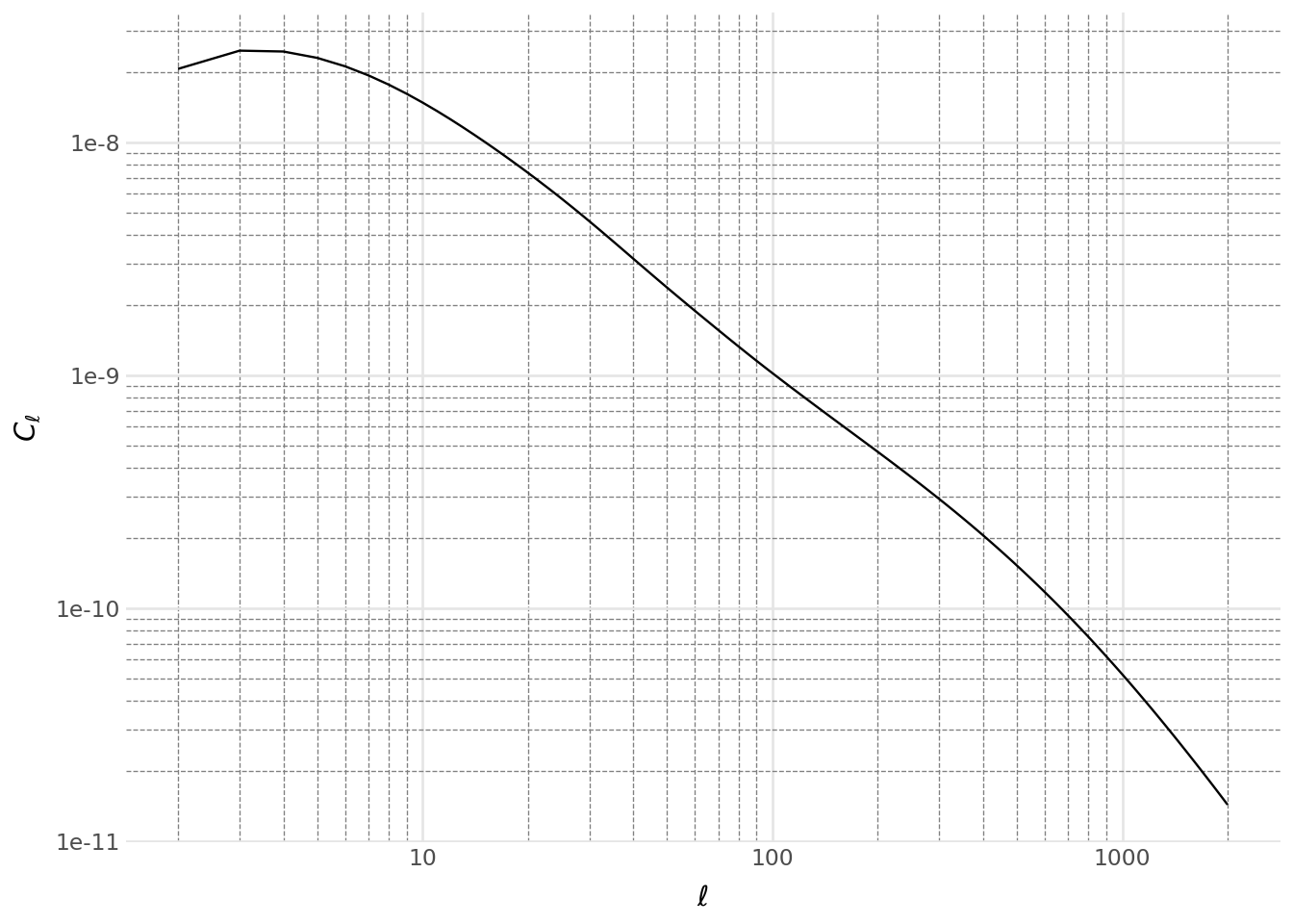
tv0 = two_point0.compute_theory_vector(tools)

Visualize the first correlation:

from plotnine import *
import pandas as pd

data = pd.DataFrame(
    {
        "ell": two_point0.ells,
        "Cell": tv0,
        "bin-x": meta0.XY.x.bin_name,
        "bin-y": meta0.XY.y.bin_name,
        "measurement": meta0.get_sacc_name(),
    }
)

(
    ggplot(data, aes("ell", "Cell"))
    + geom_line()
    + labs(x=r"$\ell$", y=r"$C_\ell$")
    + scale_x_log10()
    + scale_y_log10()
    + doc_theme()
)

Figure 1: First two-point correlation from generated metadata

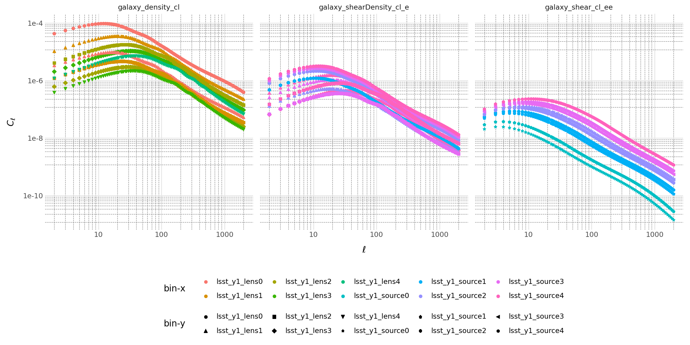
Compute all correlations:

two_point_pd_list = []
for two_point, meta in zip(all_two_point_functions, all_two_point_cells):
    two_point_pd_list.append(
        pd.DataFrame(
            {
                "ell": two_point.ells,
                "Cell": np.abs(two_point.compute_theory_vector(tools)),
                "bin-x": meta.XY.x.bin_name,
                "bin-y": meta.XY.y.bin_name,
                "measurement": meta.get_sacc_name(),
            }
        )
    )

data = pd.concat(two_point_pd_list)

(
    ggplot(data, aes("ell", "Cell", color="bin-x", shape="bin-y"))
    + geom_point()
    + labs(x=r"$\ell$", y=r"$C_\ell$")
    + scale_x_log10()
    + scale_y_log10()
    + facet_wrap("measurement")
    + doc_theme()
    + theme(
        figure_size=(12, 6),
        legend_position="bottom",
        legend_box="vertical",
    )
    + guides(
        color=guide_legend(nrow=2),
        shape=guide_legend(nrow=2),
    )
)

Complete Example: SACC Data

This example shows the full workflow starting from SACC data. For details on SACC extraction methods, see Loading SACC Data.

Using Full Extraction (Recommended)

from firecrown.data_functions import (
    extract_all_real_data,
    check_two_point_consistence_real,
)
from firecrown.likelihood.factories import load_sacc_data
from firecrown.utils import base_model_from_yaml

# Load and extract
sacc_data = load_sacc_data("../tests/sacc_data.hdf5")
two_point_reals = extract_all_real_data(sacc_data)
check_two_point_consistence_real(two_point_reals)

# Define factory via YAML
two_point_yaml = """
correlation_space: real
weak_lensing_factories:
  - type_source: default
    per_bin_systematics:
    - type: MultiplicativeShearBiasFactory
    - type: PhotoZShiftFactory
    global_systematics:
    - type: LinearAlignmentSystematicFactory
      alphag: 1.0
number_counts_factories:
  - type_source: default
    per_bin_systematics:
    - type: PhotoZShiftFactory
    global_systematics: []
"""

tp_factory = base_model_from_yaml(TwoPointFactory, two_point_yaml)
two_points_ready = TwoPoint.from_measurement(two_point_reals, tp_factory)

Create likelihood and compute:

from firecrown.likelihood import ConstGaussian
from firecrown.updatable import get_default_params_map

likelihood_ready = ConstGaussian.create_ready(
    two_points_ready, sacc_data.covariance.dense
)

# Setup and compute
tools = ModelingTools(ccl_factory=CCLFactory(require_nonlinear_pk=True))
params = get_default_params_map(tools, likelihood_ready)

tools.update(params)
tools.prepare()
likelihood_ready.update(params)

loglike = likelihood_ready.compute_loglike(tools)
print(f"Log-likelihood: {loglike}")

Log-likelihood: -2742.739024737394

Using Indices-Only Extraction (Deprecated)

from firecrown.metadata_functions import extract_all_real_metadata_indices

# Extract metadata indices
all_meta = extract_all_real_metadata_indices(sacc_data)

# Construct TwoPoint objects
two_point_list = TwoPoint.from_metadata_index(all_meta, tp_factory)

# Create likelihood and load data
likelihood = ConstGaussian(two_point_list)
likelihood.read(sacc_data)

# Prepare and compute
tools = ModelingTools(ccl_factory=CCLFactory(require_nonlinear_pk=True))
params2 = get_default_params_map(tools, likelihood)
tools.update(params2)
tools.prepare()
likelihood.update(params2)

loglike2 = likelihood.compute_loglike(tools)
print(f"Log-likelihood (legacy): {loglike2}")

Log-likelihood (legacy): -2742.739024737394

Both methods produce identical results:

import numpy as np
assert np.isclose(loglike, loglike2)
print(f"Results match: {np.isclose(loglike, loglike2)}")

Results match: True

Next Steps

Now that you understand factory construction and computation:

• Generate metadata: Two-Point Generators
• Load SACC data: Loading SACC Data
• Apply scale cuts: Scale Cuts and Filtering
• Tune computation: Integration Methods