Controlling Integration Methods

Version ?env:FIRECROWN_VERSION

def doc_theme():
    return theme_minimal() + theme(
        panel_grid_minor=element_line(color="gray", linetype="--"),
    )

Purpose of this Document

This tutorial demonstrates how to control the integration methods used when computing two-point functions in harmonic space. Different integration methods offer trade-offs between accuracy and computational cost.

For background on the factory system, see Two-Point Factory Basics. For generating two-point statistics from scratch, see Two-Point Generators.

Integration Options

TwoPointFactory objects can include integration options, allowing control over how two-point functions are computed. The example below shows how to create a TwoPointFactory with integration options that reproduce the default behavior. We also create additional TwoPointFactory objects with alternative integration configurations: ClIntegrationMethod.LIMBER with ClLimberMethod.GSL_SPLINE, ClIntegrationMethod.FKEM_AUTO, and ClIntegrationMethod.FKEM_L_LIMBER.

The lens and source redshift bin collections used for the computations are imported from the firecrown.generators module: LSST_Y1_LENS_HARMONIC_BIN_COLLECTION and LSST_Y1_SOURCE_HARMONIC_BIN_COLLECTION.

Setting Up Test Data

First, we create test data using LSST Y1 bins:

import numpy as np
from firecrown.metadata_functions import make_all_photoz_bin_combinations
from firecrown.metadata_types import TwoPointHarmonic, TwoPointCorrelationSpace
from firecrown.generators import (
    LSST_Y1_LENS_HARMONIC_BIN_COLLECTION,
    LSST_Y1_SOURCE_HARMONIC_BIN_COLLECTION,
)
from firecrown.likelihood import TwoPointFactory
from firecrown.utils import (
    base_model_from_yaml,
    ClIntegrationMethod,
    ClIntegrationOptions,
    ClLimberMethod,
)

count_bins = LSST_Y1_LENS_HARMONIC_BIN_COLLECTION.generate()
shear_bins = LSST_Y1_SOURCE_HARMONIC_BIN_COLLECTION.generate()
all_y1_bins = count_bins[:1] + shear_bins[:1]

all_two_point_xy = make_all_photoz_bin_combinations(all_y1_bins)
ells = np.unique(
    np.concatenate((np.arange(2, 120), np.geomspace(120, 2000, 128)))
).astype(int)
all_two_point_cells = [TwoPointHarmonic(XY=xy, ells=ells) for xy in all_two_point_xy]

Creating Factories with Different Integration Methods

Now we create a base factory configuration and then define factories with different integration methods:

two_point_yaml = """
correlation_space: harmonic
weak_lensing_factories:
  - type_source: default
    per_bin_systematics: []
    global_systematics: []
number_counts_factories:
  - type_source: default
    per_bin_systematics: []
    global_systematics: []
"""

tpf = base_model_from_yaml(TwoPointFactory, two_point_yaml)

tpf_gsl_quad = TwoPointFactory(
    correlation_space=TwoPointCorrelationSpace.HARMONIC,
    weak_lensing_factories=tpf.weak_lensing_factories,
    number_counts_factories=tpf.number_counts_factories,
    int_options=ClIntegrationOptions(
        method=ClIntegrationMethod.LIMBER, limber_method=ClLimberMethod.GSL_QAG_QUAD
    ),
)

tpf_gsl_spline = TwoPointFactory(
    correlation_space=TwoPointCorrelationSpace.HARMONIC,
    weak_lensing_factories=tpf.weak_lensing_factories,
    number_counts_factories=tpf.number_counts_factories,
    int_options=ClIntegrationOptions(
        method=ClIntegrationMethod.LIMBER, limber_method=ClLimberMethod.GSL_SPLINE
    ),
)

tpf_fkem_auto = TwoPointFactory(
    correlation_space=TwoPointCorrelationSpace.HARMONIC,
    weak_lensing_factories=tpf.weak_lensing_factories,
    number_counts_factories=tpf.number_counts_factories,
    int_options=ClIntegrationOptions(
        method=ClIntegrationMethod.FKEM_AUTO, limber_method=ClLimberMethod.GSL_QAG_QUAD
    ),
)

tpf_fkem_l_limber = TwoPointFactory(
    correlation_space=TwoPointCorrelationSpace.HARMONIC,
    weak_lensing_factories=tpf.weak_lensing_factories,
    number_counts_factories=tpf.number_counts_factories,
    int_options=ClIntegrationOptions(
        method=ClIntegrationMethod.FKEM_L_LIMBER,
        limber_method=ClLimberMethod.GSL_QAG_QUAD,
        l_limber=50,
    ),
)

tpf_fkem_l_limber_max = TwoPointFactory(
    correlation_space=TwoPointCorrelationSpace.HARMONIC,
    weak_lensing_factories=tpf.weak_lensing_factories,
    number_counts_factories=tpf.number_counts_factories,
    int_options=ClIntegrationOptions(
        method=ClIntegrationMethod.FKEM_L_LIMBER,
        limber_method=ClLimberMethod.GSL_QAG_QUAD,
        l_limber=2100,
    ),
)

two_points_gsl_quad = tpf_gsl_quad.from_metadata(all_two_point_cells)
two_points_gsl_spline = tpf_gsl_spline.from_metadata(all_two_point_cells)
two_points_fkem_auto = tpf_fkem_auto.from_metadata(all_two_point_cells)
two_points_fkem_l_limber = tpf_fkem_l_limber.from_metadata(all_two_point_cells)
two_points_fkem_l_limber_max = tpf_fkem_l_limber_max.from_metadata(all_two_point_cells)

Computing and Comparing Results

Now we compute theory vectors with each integration method and compare the relative differences:

from firecrown.modeling_tools import ModelingTools
from firecrown.updatable import get_default_params_map

tools = ModelingTools()

two_point0_gsl_quad = two_points_gsl_quad[0]
two_point0_gsl_spline = two_points_gsl_spline[0]
two_point0_fkem_auto = two_points_fkem_auto[0]
two_point0_fkem_l_limber = two_points_fkem_l_limber[0]
two_point0_fkem_l_limber_max = two_points_fkem_l_limber_max[0]
meta0 = all_two_point_cells[0]

two_point0_gsl_quad.update(get_default_params_map(two_point0_gsl_quad))
two_point0_gsl_spline.update(get_default_params_map(two_point0_gsl_spline))
two_point0_fkem_auto.update(get_default_params_map(two_point0_fkem_auto))
two_point0_fkem_l_limber.update(get_default_params_map(two_point0_fkem_l_limber))
two_point0_fkem_l_limber_max.update(
    get_default_params_map(two_point0_fkem_l_limber_max)
)

tools.update(get_default_params_map(tools))
tools.prepare()

tv0_gsl_quad = two_point0_gsl_quad.compute_theory_vector(tools)
tv0_gsl_spline = two_point0_gsl_spline.compute_theory_vector(tools)
tv0_fkem_auto = two_point0_fkem_auto.compute_theory_vector(tools)
tv0_fkem_l_limber = two_point0_fkem_l_limber.compute_theory_vector(tools)
tv0_fkem_l_limber_max = two_point0_fkem_l_limber_max.compute_theory_vector(tools)

/home/docs/checkouts/readthedocs.org/user_builds/firecrown/conda/v1.15.0/lib/python3.14/site-packages/pyccl/errors.py:22: CCLWarning: Nchi must be a positive integer. Setting to match tracer with large chi samples x 2.
  warnings_builtin.warn(*args, **kwargs)
/home/docs/checkouts/readthedocs.org/user_builds/firecrown/conda/v1.15.0/lib/python3.14/site-packages/pyccl/errors.py:22: CCLWarning: chi_min must be greater than zero.Setting to default 1e-6 Mpc.
  warnings_builtin.warn(*args, **kwargs)

Visualizing Differences

Now we plot the relative differences between each integration method and the most accurate (FKEM applied to all ells), highlighting the impact of different integration choices on the two-point functions:

from plotnine import *
import pandas as pd

tmp = np.abs(tv0_gsl_spline / tv0_fkem_l_limber_max - 1.0)
data_gsl_spline = pd.DataFrame(
    {
        "ell": two_point0_gsl_spline.ells[tmp > 0.0],
        "rel-diff": tmp[tmp > 0.0],
        "bin-x": meta0.XY.x.bin_name,
        "bin-y": meta0.XY.y.bin_name,
        "measurement": meta0.get_sacc_name(),
        "integration": "GSL SPLINE",
    }
)

tmp = np.abs(tv0_gsl_quad / tv0_fkem_l_limber_max - 1.0)
data_gsl_quad = pd.DataFrame(
    {
        "ell": two_point0_gsl_quad.ells[tmp > 0.0],
        "rel-diff": tmp[tmp > 0.0],
        "bin-x": meta0.XY.x.bin_name,
        "bin-y": meta0.XY.y.bin_name,
        "measurement": meta0.get_sacc_name(),
        "integration": "GSL QAG_QUAD",
    }
)

tmp = np.abs(tv0_fkem_auto / tv0_fkem_l_limber_max - 1.0)
data_fkem_auto = pd.DataFrame(
    {
        "ell": two_point0_fkem_auto.ells[tmp > 0.0],
        "rel-diff": tmp[tmp > 0.0],
        "bin-x": meta0.XY.x.bin_name,
        "bin-y": meta0.XY.y.bin_name,
        "measurement": meta0.get_sacc_name(),
        "integration": "FKEM AUTO",
    }
)

tmp = np.abs(tv0_fkem_l_limber / tv0_fkem_l_limber_max - 1.0)
data_fkem_l_limber = pd.DataFrame(
    {
        "ell": two_point0_fkem_l_limber.ells[tmp > 0.0],
        "rel-diff": tmp[tmp > 0.0],
        "bin-x": meta0.XY.x.bin_name,
        "bin-y": meta0.XY.y.bin_name,
        "measurement": meta0.get_sacc_name(),
        "integration": "FKEM l-limber (50)",
    }
)

data = pd.concat([data_gsl_spline, data_gsl_quad, data_fkem_auto, data_fkem_l_limber])

(
    ggplot(data, aes("ell", "rel-diff"))
    + geom_line()
    + labs(x=r"$\ell$", y=r"$|C^X_\ell/C^\mathrm{reference}_\ell - 1|$")
    + scale_x_log10()
    + scale_y_log10()
    + doc_theme()
    + facet_wrap("integration")
    + theme(figure_size=(10, 6))
)

Figure 1: Relative difference compared to FKEM with maximum l_limber

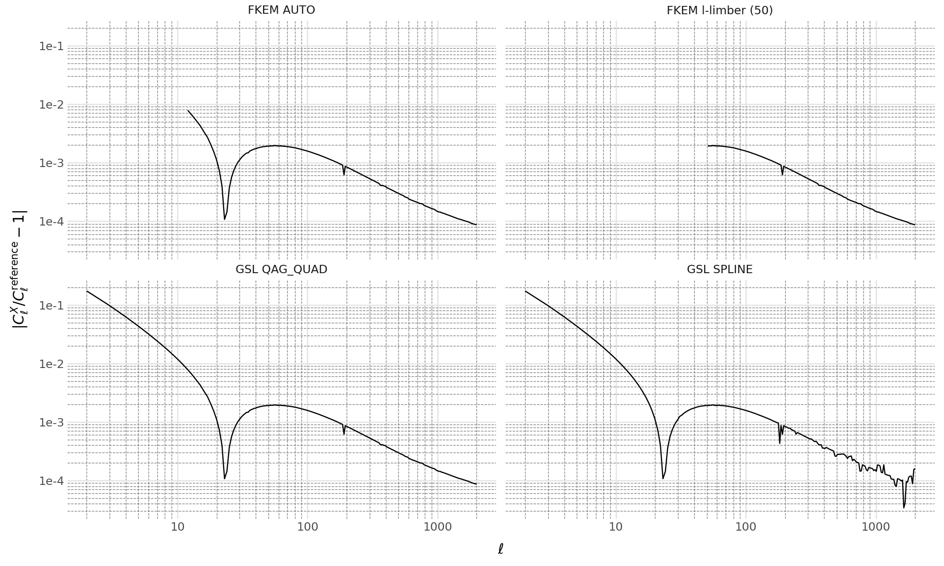
The plot shows that different integration methods produce varying levels of accuracy. The FKEM methods generally provide better accuracy, especially at low \(\ell\) values, while the Limber approximation with GSL methods may introduce larger errors at small scales.

Summary

This tutorial demonstrated:

• How to configure different integration methods using ClIntegrationOptions
• The available integration methods: LIMBER, FKEM_AUTO, and FKEM_L_LIMBER
• How to compare accuracy across different methods
• The trade-offs between computational cost and accuracy

For most analyses, the default settings provide a good balance. Use more accurate methods (like FKEM_L_LIMBER with high l_limber) when precision is critical at low multipoles.